Outline IAML: Overfitting and Capacity Control Generalization error - PowerPoint PPT Presentation
Outline IAML: Overfitting and Capacity Control Generalization error Estimating generalization error Example: polynomial regression Charles Sutton and Victor Lavrenko School of Informatics Under- and over-fitting
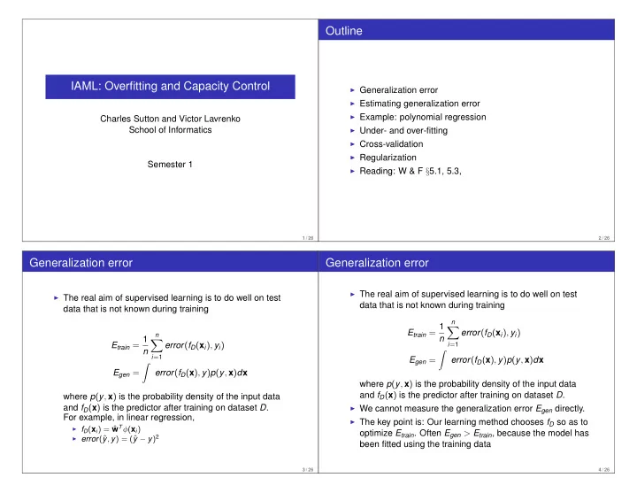
Outline IAML: Overfitting and Capacity Control ◮ Generalization error ◮ Estimating generalization error ◮ Example: polynomial regression Charles Sutton and Victor Lavrenko School of Informatics ◮ Under- and over-fitting ◮ Cross-validation ◮ Regularization Semester 1 ◮ Reading: W & F § 5.1, 5.3, 1 / 26 2 / 26 Generalization error Generalization error ◮ The real aim of supervised learning is to do well on test ◮ The real aim of supervised learning is to do well on test data that is not known during training data that is not known during training n E train = 1 � error ( f D ( x i ) , y i ) n E train = 1 n � error ( f D ( x i ) , y i ) i = 1 n � i = 1 E gen = error ( f D ( x ) , y ) p ( y , x ) d x � E gen = error ( f D ( x ) , y ) p ( y , x ) d x where p ( y , x ) is the probability density of the input data and f D ( x ) is the predictor after training on dataset D . where p ( y , x ) is the probability density of the input data and f D ( x ) is the predictor after training on dataset D . ◮ We cannot measure the generalization error E gen directly. For example, in linear regression, ◮ The key point is: Our learning method chooses f D so as to ◮ f D ( x i ) = ˆ w T φ ( x i ) optimize E train . Often E gen > E train , because the model has ◮ error (ˆ y − y ) 2 y , y ) = (ˆ been fitted using the training data 3 / 26 4 / 26
Polynomial regression Under- and Overfitting φ ( x ) = ( 1 , x , x 2 , . . . , x M ) T ◮ Choosing values of the parameters that minimize the training error may not lead to the best generalization 1 M = 0 1 M = 1 t t performance 0 0 ◮ If the model too simple, it will not be able to represent the patterns that exist. This is underfitting . −1 −1 ◮ If the model is too complex, it will memorize the training 0 1 0 1 x x data. It will remember “noise”, i.e., patterns in the data that occur only due to chance. This is called overfitting . 1 M = 3 1 M = 9 ◮ Overfitting: A hypothesis f ∈ F is said to overfit the data if t t there exists some alternative hypothesis f ′ ∈ F such that f 0 0 has a smaller training error than f ′ , but f ′ has a smaller generalization error than f . −1 −1 ◮ Need a balance between the two 0 1 0 1 x x Figure credit: Chris Bishop, PRML 5 / 26 6 / 26 Training vs Generalization Error Knobs are your friend ◮ Every data set will require a different balance between over- and underfitting. Depends on how much data we have and how complex the actual relationship is ◮ In general we need: (a) a knob that causes the algorithm to favour simpler or more complex rules, and (b) a procedure for setting this knob based on data, to choose the right balance ◮ This is why all the learning algorithms in Weka have parameters. ◮ For decision trees: The parameters of the pruning algorithm ◮ For polynomial regression: M (order of the polynomial) Adapted from figure by Sam Roweis. ◮ For k -nearest neighbor: 7 / 26 8 / 26
Knobs are your friend Knobs are your friend ◮ Every data set will require a different balance between ◮ Every data set will require a different balance between over- and underfitting. Depends on how much data we over- and underfitting. Depends on how much data we have and how complex the actual relationship is have and how complex the actual relationship is ◮ In general we need: (a) a knob that causes the algorithm ◮ In general we need: (a) a knob that causes the algorithm to favour simpler or more complex rules, and (b) a to favour simpler or more complex rules, and (b) a procedure for setting this knob based on data, to choose procedure for setting this knob based on data, to choose the right balance the right balance ◮ This is why all the learning algorithms in Weka have ◮ This is why all the learning algorithms in Weka have parameters. parameters. ◮ For decision trees: The parameters of the pruning ◮ For decision trees: The parameters of the pruning algorithm algorithm ◮ For polynomial regression: M (order of the polynomial) ◮ For polynomial regression: M (order of the polynomial) ◮ For k -nearest neighbor: k ◮ For k -nearest neighbor: k ◮ For linear regression: ◮ For linear regression: ???? 9 / 26 10 / 26 Regularization Regularized Loss Function ◮ Regularization is a general approach to add a “complexity knob” to a learning algorithm. Requires that the parameters be continuous. (i.e., Regression OK, Decision ◮ The overall cost function is the trees not.) sum of two parabolic bowls. ◮ If we penalize polynomials that have large values for their The sum is also a parabolic bowl. coefficients we will get less wiggly solutions ◮ The combined minimum lies E ( w ) = | y − Φ w | 2 + λ | w | 2 ˜ on the line between the minimum of the squared error ◮ Solution is and the origin. w = (Φ T Φ + λ I ) − 1 Φ T y ˆ ◮ The regularizer just shrinks ◮ This is known as ridge regression the weights. ◮ Rather than using a discrete control parameter like M (model order) we can use a continuous parameter λ Credit: Geoff Hinton ◮ Caution: Don’t shrink the bias term! (The one that corresponds to the all 1 feature.) 11 / 26 12 / 26
The effect of regularization for M = 9 M = 9 1 ln λ = − 18 1 M = 9 1 Training t t Test 0 0 −1 −1 E RMS 0.5 0 1 0 1 x x 1 ln λ = 0 t 0 0 −35 −30 −25 −20 ln λ −1 Chris Bishop, PRML 0 1 x Figure credit: Chris Bishop, PRML 13 / 26 14 / 26 But with ridge regression we have For regular old linear regression, we had ◮ Define the task : regression ◮ Decide on the model structure : linear regression model ◮ Define the task : regression ◮ Decide on the score function : squared error with ◮ Decide on the model structure : linear regression model quadratic regularizaton ◮ Decide on the score function : squared error (likelihood) ◮ Decide on optimization/search method to optimize the ◮ Decide on optimization/search method to optimize the score function: calculus (analytic solution) score function: calculus (analytic solution) Notice how you can train the same model structure with different score functions. This is the first time we have seen this. This is important. 15 / 26 16 / 26
A Knob-Setting Procedure Using a validation set ◮ Split the labelled data into a training set, validation set, and ◮ Regularization was a way of adding “capacity control” a a test set. knob. ◮ Training set: Use for training ◮ But how do we set the value? e.g., the regularization ◮ Validation set: Tune the “knobs” according to performance parameter λ on the validation set ◮ Won’t work to do it on the training set (why not?) ◮ Test set: to check how the final model performs ◮ We will cover two choices ◮ Validation set ◮ No right answers, but for example, could choose 60% ◮ Cross-validation training, 20% validation, 20% test 17 / 26 18 / 26 Example of using a validation set Cross-validation Consider polynomial regression: 1. For each m = 1 , 2 , . . . M (you choose M in advance 2. Train the polynomial regression using ◮ The idea of holding out a separate validation set seems φ ( x ) = ( 1 , x , x 2 , . . . , x m ) T on training set (e.g., by rather wasteful of data → k -fold cross validation. minimizing squared error). This produces a predictor f m ( x ) . ◮ Divide the labelled data into k parts (or folds), train on k − 1 3. Measure the error of f m on the validation set folds, and validate on one. Do this k times, holding out a 4. End for different fold each time. Common choices for k are 3 or 10 5. Choose the f m with the best validation error. 6. Measure the error of f m on the test set to see how well you should expect it to perform 19 / 26 20 / 26
Cross-validation (pretty) Cross-validation ◮ Validation performance is average of validation 1 5 1 1 performance on each of the k folds Test Train ◮ Choose m with the maximum validation performance 2-5 Train 4 2 Test ◮ If k = n , then we have leave-one-out cross validation 2 Train 3-5 Test (LOO-CV) 3 ◮ Once you have selected m , pool all of the data back Fold 1 Fold 2 Fold 3 together, train as usual on that value only. 21 / 26 22 / 26 Continuous Knobs Continuous Knobs ◮ For a discrete knob like polynomial order m we could ◮ For a discrete knob like polynomial order m we could simply search all values. simply search all values. ◮ What about a quadratic regularization parameter λ . What ◮ What about a quadratic regularization parameter λ . What do we do then? do we do then? ◮ Pick a grid of values to search. In practice you want the grid to vary geometrically for this sort of parameter. e.g., Try λ ∈ { 0 . 01 , 0 . 1 , 0 . 5 , 1 . 0 , 5 . 0 , 10 . 0 } . Don’t bother trying 2 . 0, 3 . 0, 7 . 0. 23 / 26 24 / 26
Problems with cross-validation Summary ◮ You can still overfit! If you exhaustively try a really large ◮ Generalization error vs training error number of possible approaches and knob settings, you ◮ Under- and over-fitting could by chance happen to find a parameter setting that ◮ Using knobs to control the complexity of a predictor predicts all the training data well. ◮ Estimate generalization error with a validation set (or CV) ◮ It can be expensive computationally. ◮ Regularization ◮ Sometimes there are tricks to reduce the computation. 25 / 26 26 / 26
Recommend
More recommend
Explore More Topics
Stay informed with curated content and fresh updates.
