IAML: Optimization Charles Sutton and Victor Lavrenko School of - PowerPoint PPT Presentation
IAML: Optimization Charles Sutton and Victor Lavrenko School of Informatics Semester 1 1 / 24 Outline Why we use optimization in machine learning The general optimization problem Gradient descent Problems with gradient descent
IAML: Optimization Charles Sutton and Victor Lavrenko School of Informatics Semester 1 1 / 24
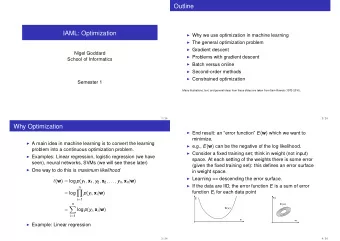
Outline ◮ Why we use optimization in machine learning ◮ The general optimization problem ◮ Gradient descent ◮ Problems with gradient descent ◮ Batch versus online ◮ Second-order methods ◮ Constrained optimization Many illustrations, text, and general ideas from these slides are taken from Sam Roweis (1972-2010). 2 / 24
Why Optimization ◮ A main idea in machine learning is to convert the learning problem in a continuous optimization problem. ◮ Examples: Linear regression, logistic regression (we have seen), neural networks, SVMs (we will see these later) ◮ One way to do this is maximum likelihood ℓ ( w ) = log p ( y 1 , x 1 , y 2 , x 2 , . . . , y n , x n | w ) n � = log p ( y i , x i | w ) i = 1 n � = log p ( y i , x i | w ) i = 1 ◮ Example: Linear regression 3 / 24
◮ End result: an “error function” E ( w ) which we want to minimize. ◮ e.g., E ( w ) can be the negative of the log likelihood. ◮ Consider a fixed training set; think in weight (not input) space. At each setting of the weights there is some error (given the fixed training set): this defines an error surface in weight space. ◮ Learning == descending the error surface. ◮ If the data are IID, the error function E is a sum of error function E i for each data point wj E E(w) E(w) w wi 4 / 24
Role of Smoothness If E completely unconstrained, minimization is impossible. E(w) w All we could do is search through all possible values w . Key idea: If E is continuous, then measuring E ( w ) gives information about E at many nearby values. 5 / 24
Role of Derivatives ◮ If we wiggle w k and keep everything else the same, does the error get better or worse? ◮ Calculus has an answer to exactly this question: ∂ E ∂ w k ◮ So: use a differentiable cost function E and compute partial derivatives of each parameter ◮ The vector of partial derivatives is called the gradient of the error. It is written ∇ E = ( ∂ E ∂ w 1 , ∂ E ∂ w 2 , . . . , ∂ E ∂ w n ) . Alternate notation ∂ E ∂ w . ◮ It points in the direction of steepest error descent in weight space. ◮ Three crucial questions: ◮ How do we compute the gradient ∇ E efficiently? ◮ Once we have the gradient, how do we minimize the error? ◮ Where will we end up in weight space? 6 / 24
Numerical Optimization Algorithms ◮ Numerical optimization algorithms try to solve the general problem min w E ( w ) ◮ Most commonly, a numerical optimization procedure takes two inputs: ◮ A procedure that computes E ( w ) ◮ A procedure that computes the partial derivative ∂ E ∂ w j ◮ (Aside: Some use less information, i.e., they don’t use gradients. Some use more information, i.e., higher order derivative. We won’t go into these algorithms in the course.) 7 / 24
Optimization Algorithm Cartoon ◮ Basically, numerical optimization algorithms are iterative. They generate a sequence of points w 0 , w 1 , w 2 , . . . E ( w 0 ) , E ( w 1 ) , E ( w 2 ) , . . . ∇ E ( w 0 ) , ∇ E ( w 1 ) , ∇ E ( w 2 ) , . . . ◮ Basic optimization algorithm is initialize w while E ( w ) is unacceptably high calculate g = ∇ E Compute direction d from w , E ( w ) , g (can use previous gradients as well...) w ← w − η d end while return w 8 / 24
A Choice of Direction ◮ The simplest choice d is the current gradient ∇ E . ◮ It is locally the steepest descent direction. ◮ (Technically, the reason for this choice is Taylor’s theorem from calculus.) 9 / 24
Gradient Descent ◮ Simple gradient descent algorithm: initialize w while L ( w ) is unacceptably high calculate g ← ∂ E ∂ w w ← w − η g end while return w ◮ η is known as the step size (sometimes called learning rate ) ◮ We must choose η > 0. ◮ η too small → too slow ◮ η too large → instability 10 / 24
Effect of Step Size Goal: Minimize E ( w ) = w 2 ◮ Take η = 0 . 1. Works good. 8 w 0 = 1 . 0 6 w 1 = w 0 − 0 . 1 · 2 w 0 = 0 . 8 E(w) 4 w 2 = w 1 − 0 . 1 · 2 w 1 = 0 . 64 w 3 = w 2 − 0 . 1 · 2 w 2 = 0 . 512 2 · · · 0 w 25 = 0 . 0047 −3 −2 −1 0 1 2 3 w 11 / 24
Effect of Step Size ◮ Take η = 1 . 1. Not so good. If you Goal: Minimize step too far, you can leap over the E ( w ) = w 2 region that contains the minimum 8 w 0 = 1 . 0 6 w 1 = w 0 − 1 . 1 · 2 w 0 = − 1 . 2 E(w) w 2 = w 1 − 1 . 1 · 2 w 1 = 1 . 44 4 w 3 = w 2 − 1 . 1 · 2 w 2 = − 1 . 72 2 · · · 0 w 25 = 79 . 50 −3 −2 −1 0 1 2 3 ◮ Finally, take η = 0 . 000001. What w happens here? 12 / 24
“Bold Driver” Gradient Descent ◮ Simple heuristic for choosing η which you can use if you’re desperate. initialize w , η initialize e ← E ( w ) ; g ← ∇ E ( w ) while η > 0 w 1 ← w − η g e 1 = E ( w 1 ) ; g 1 = ∇ E if e 1 ≥ e η = η/ 2 else η = 1 . 01 η ; w ← w 1 ; g = g 1 end while return w ◮ Finds a local minimum of E . 13 / 24
Batch vs online ◮ So far all the objective function we have seen look like: n � E ( w ; D ) = E i ( w ; y i , x i ) . i = 1 D = { ( x 1 , y 1 ) , ( x 2 , y 2 ) , . . . ( x n , y n ) } is the training set. ◮ Each term sum depends on only one training instance ◮ Example: Logistic regression: E i ( w ; y i , x i ) = log p ( y i | x i , w ) . ◮ The gradient in this case is always n ∂ E ∂ E i � ∂ w = ∂ w i = 1 ◮ The algorithm on slide 10 scans all the training instances before changing the parameters. ◮ Seems dumb if we have millions of training instances. Surely we can get a gradient that is “good enough” from fewer instances, e.g., a couple thousand? Or maybe even from just one? 14 / 24
Batch vs online ◮ Batch learning: use all patterns in training set, and update weights after calculating ∂ E ∂ E i � ∂ w = ∂ w i ◮ On-line learning: adapt weights after each pattern presentation, using ∂ E i ∂ w ◮ Batch more powerful optimization methods ◮ Batch easier to analyze ◮ On-line more feasible for huge or continually growing datasets ◮ On-line may have ability to jump over local optima 15 / 24
Algorithms for Batch Gradient Descent ◮ Here is batch gradient descent. initialize w while E ( w ) is unacceptably high calculate g ← � N ∂ E i i = 1 ∂ w w ← w − η g end while return w ◮ This is just the algorithm we have seen before. We have just “substituted in” the fact that E = � N i = 1 E i . 16 / 24
Algorithms for Online Gradient Descent ◮ Here is (a particular type of) online gradient descent algorithm initialize w while E ( w ) is unacceptably high Pick j as uniform random integer in 1 . . . N calculate g ← ∂ E j ∂ w w ← w − η g end while return w ◮ This version is also called “stochastic gradient ascent” because we have picked the training instance randomly. ◮ There are other variants of online gradient descent. 17 / 24
Problems With Gradient Descent ◮ Setting the step size η ◮ Shallow valleys ◮ Highly curved error surfaces ◮ Local minima 18 / 24
Shallow Valleys ◮ Typical gradient descent can be fooled in several ways, which is why more sophisticated methods are used when possible. One problem: quickly down the valley walls but very slowly along the valley bottom. dE dw ◮ Gradient descent goes very slowly once it hits the shallow valley. ◮ One hack to deal with this is momentum d t = β d t − 1 + ( 1 − β ) η ∇ E ( w t ) ◮ Now you have to set both η and β . Can be difficult and irritating. 19 / 24
Curved Error Surfaces ◮ A second problem with gradient descent is that the gradient might not point towards the optimum. This is because of curvature directly at the nearest local minimum. dE dW ◮ Note: gradient is the locally steepest direction. Need not directly point toward local optimum. ◮ Local curvature is measured by the Hessian matrix: H ij = ∂ 2 E /∂ w i w j . ◮ By the way, do these ellipses remind you of anything? 20 / 24
Local Minima ◮ If you follow the gradient, where will you end up? Once you hit a local minimum, gradient is 0, so you stop. error parameter space ◮ Certain nice functions, such as squared error, logistic regression likelihood are convex , meaning that the second derivative is always positive. This implies that any local minimum is global. ◮ There is no great solution to this problem. It is fundamentally one. Usually, the best you can do is rerun the optimizer multiple times from different random starting points. 21 / 24
Advanced Topics That We Will Not Cover (Part I) ◮ Some of these issues (shallow valley, curved error surfaces) can be fixed ◮ Some of these are second-order methods like Newton’s method that use the second derivatives ◮ Also there are fancy first-order methods like quasi-Newton methods (I like one called limited memory BFGS ) and conjugate gradient ◮ They are the state of the art methods for logistic regression (as long as there are not too many data points) ◮ We will not discuss these methods in the course. ◮ Other issues (like local minima) cannot be easily fixed 22 / 24
Recommend
More recommend
Explore More Topics
Stay informed with curated content and fresh updates.
