[PDF] - CS 4100: Artificial Intelligence Optimization and Neural Nets PDF Document

SLIDE 1

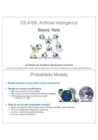
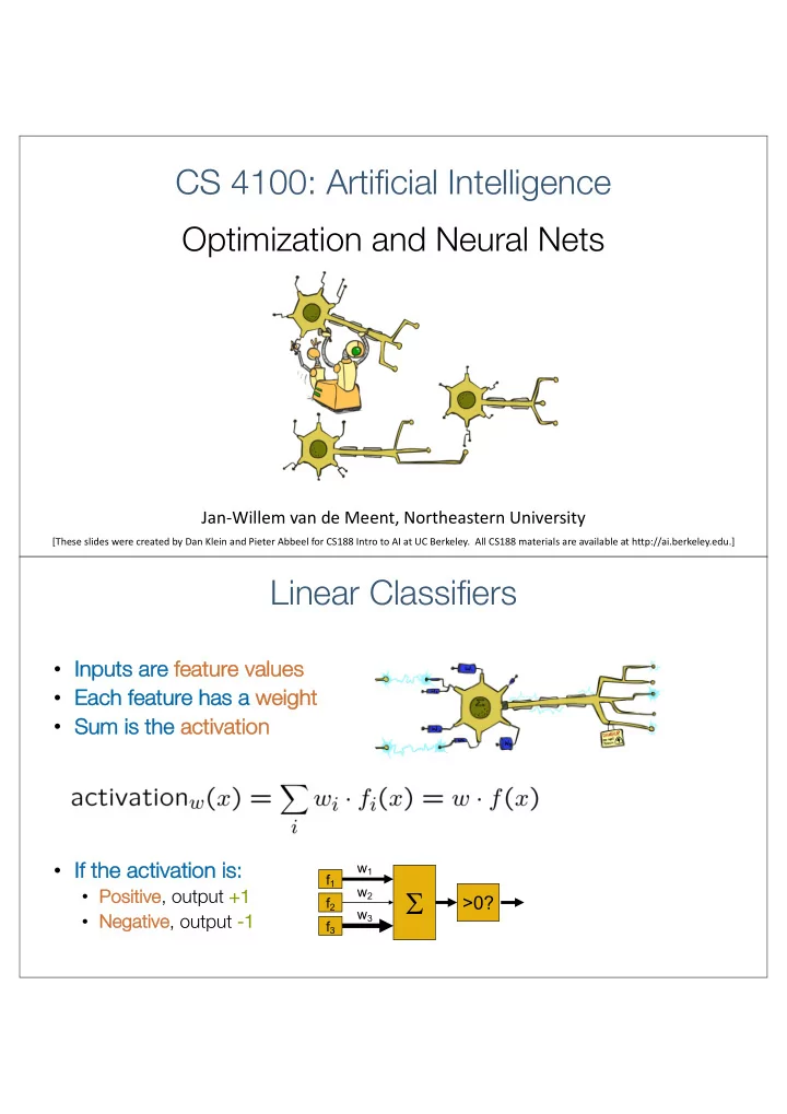
CS 4100: Artificial Intelligence

Optimization and Neural Nets

Jan-Willem van de Meent, Northeastern University

[These slides were created by Dan Klein and Pieter Abbeel for CS188 Intro to AI at UC Berkeley. All CS188 materials are available at http://ai.berkeley.edu.]

Linear Classifiers

In

Inputs s are fe feature values

Ea

Each feature has s a we weight

Su

Sum is the act activat ation

If

If the activa vation is: s:

Po

Positive ve, output +1 +1

Ne

Negative, output -1

S

f1 f2 f3 w1 w2 w3

>0?

SLIDE 2

How to get probabilistic decisions?

Ac

Activ ivation ion:

If

If very po positive à want probability going to 1

If

If very ne negative ive à want probability going to 0

Sigmoid

Sigmoid fu function ion

z = w · f(x)

z = w · f(x) z = w · f(x)

φ(z) = 1 1 + e−z

Best w?

Maximum like

kelihood estimation: wi with th:

max

w

ll(w) = max

w

X

i

log P(y(i)|x(i); w) P(y(i) = +1|x(i); w) = 1 1 + e−w·f(x(i)) P(y(i) = −1|x(i); w) = 1 − 1 1 + e−w·f(x(i))

Th This is is is calle lled Lo Logis istic ic Regressio ion

SLIDE 3

Multiclass Logistic Regression

Re

Recall Perceptron: n:

A we

weig ight vector for each class:

Sc

Score (activation) of a class y:

Prediction with hi

highe ghest st sc scor

re wins

ns

Ho

How w to tur urn n sc scores s in into pr proba babi bilities? ?

z1, z2, z3 → ez1 ez1 + ez2 + ez3 , ez2 ez1 + ez2 + ez3 , ez3 ez1 + ez2 + ez3

riginal activations

softmax activations

Best w?

Maximum like

kelihood estimation: wi with th:

max

w

ll(w) = max

w

X

i

log P(y(i)|x(i); w) P(y(i)|x(i); w) = ewy(i)·f(x(i)) P

y ewy·f(x(i))

Th This is is is calle lled Mu Multi-Cl Class L ss Logist stic R Regressi ssion

SLIDE 4

This Lecture

Op

Opti timizati tion

i.e., how do we solve:

max

w

ll(w) = max

w

X

i

log P(y(i)|x(i); w)

Hill Climbing

Re

Recall fro rom CSPs lectu ture re: simple, general idea

St

Start wherever

Re

Repeat: move to the best neighboring state

If no neighbors better than current, quit
What’s particularly tricky

ky when hill-cl climbi bing for for mu mult ltic icla lass logis logistic ic regr gression ion?

Optimization over a co

continuous s space ace

Infinitely many neighbors!
How to do this efficiently?

SLIDE 5

1-D Optimization

Co

Could ev eval aluate ate an and

Then step in be

best di dire rection

n
Or,

Or, evaluate te der derivat ative

Defines di

dire rection

n to step into

w

g(w)

w0 g(w0)

g(w0 + h)

g(w0 − h)

∂g(w0) ∂w = lim

h→0

g(w0 + h) − g(w0 − h) 2h

2-D Optimization

Source: offconvex.org

SLIDE 6

Gradient Ascent

Pe

Perfo form update in uphill direction fo for each coordinate

The steeper the slope (i.e. the higher the derivative)

the bigger the step for that coordinate

E.

E.g., consi sider:

Up

Updates:

g(w1, w2)

w2 ← w2 + α ∗ @g @w2 (w1, w2) w1 ← w1 + α ∗ @g @w1 (w1, w2)

Up

Updates in in vector r notatio ion:

with:

w ← w + α ∗ rwg(w)

rwg(w) = "

∂g ∂w1 (w) ∂g ∂w2 (w)

# = = gradient

Gradient Ascent

Id

Idea:

St

Start somewhere

Re

Repeat: Take a step in the gradient direction

Figure source: Mathworks

SLIDE 7

What is the Steepest Direction?

Fi

First-Or Orde der Taylor Expa pansion:

St

Steepest Asc scent Dire Directio ion:

Re

Recall: à

He

Henc nce, solut ution: n:

g(w + ∆) ≈ g(w) + ∂g ∂w1 ∆1 + ∂g ∂w2 ∆2

rg = "

∂g ∂w1 ∂g ∂w2

#

Gr Gradi dient di direction = = steepe pest di direction!

max

∆:∆2

1+∆2 2≤ε

g(w + ∆)

max

∆:∆2

1+∆2 2≤ε

g(w) + ∂g ∂w1 ∆1 + ∂g ∂w2 ∆2

∆ = ε rg krgk

∆ = ε a kak max

∆:k∆k≤ε ∆>a

|Δ| ≤ ε1/2 w a Δ

Gradient in n dimensions

rg =     

∂g ∂w1 ∂g ∂w2

· · ·

∂g ∂wn

    

SLIDE 8

Optimization Procedure: Gradient Ascent

initialize
for iter = 1, 2, …

w

le

learning ning ra rate te - hyperparameter that needs to be chosen carefully

Ho

How? Try multiple choices

Cr

Crude rule of thumb mb: update changes about 0. 0.1 1 – 1% 1%

α w w ← w + α ∗ rg(w)

Gradient Ascent on the Log Likelihood Objective

initialize
for iter = 1, 2, …

max

w

ll(w) = max

w

X

i

log P(y(i)|x(i); w)

g(w) w

w ← w + α ∗ X

i

r log P(y(i)|x(i); w)

(Sum over al all training examples)

SLIDE 9

St Stoch chast astic c Gradient Ascent on the Log Likelihood Objective

initialize
for iter = 1, 2, …
pick random j

max

w

ll(w) = max

w

X

i

log P(y(i)|x(i); w) w

w ← w + α ∗ r log P(y(j)|x(j); w)

Obs Observation: once the gradient on one training example has been computed, we might as well incorporate before computing next one In Intuition: Use sampling to approximate the gradient. This is called st stochast stic g gradient d desc scent.

Mi Mini-Ba Batch Gradient Ascent on the Log Likelihood Objective

initialize
for iter = 1, 2, …
pick random subset of training examples J

max

w

ll(w) = max

w

X

i

log P(y(i)|x(i); w) w

Obs Observation: gradient over small set of training examples (=m =mini-ba batch) can be computed in parallel, might as well do that instead of a single one

w ← w + α ∗ X

j∈J

r log P(y(j)|x(j); w)

SLIDE 10

How about computing all the derivatives?

We’ll talk about that once we covered neural networks,

which are a generalization of logistic regression

Neural Networks

SLIDE 11

Multi-class Logistic Regression

Lo

Logis istic ic regressio ion n is is a specia ial l case of

f a

a ne neur ural l ne network

z1 z2 z3

f1(x) f2(x) f3(x) fK(x)

s

f

t m a x

P(y1|x; w) = ez1 ez1 + ez2 + ez3 P(y2|x; w) = ez2 ez1 + ez2 + ez3

P(y3|x; w) = ez3 ez1 + ez2 + ez3

…

W1,

1,1

W1,

1,2

W1,

1,3

W3,3

,3

zi = X

j

Wi,j fj(x)

<latexit sha1_base64="5jPDuadc92/H0mDYLheYrIDBNTY=">AHNnicfZXPb9MwFMe9AWUXxsckVBFhzSkqkrW0Y1JSNPGNG6MiW1ITVU5idumdX5gO107yzf+Gq5w4F/hwg1x5U/ATgIkcZijNZ7n/f1s/ts2xH2KDOMb0vL167fqN1cuVW/fefuvfuraw/OaBgTB506IQ7JextShL0AnTKPYfQ+Igj6Nkbn9vRA+c9niFAvDN6xRYT6PhwF3tBzIJOmwerjy4HXeNmwaOwPJo3zAfdaE9GwdhvDwWRj/myw2jTaRtIaesfMOs09kLbjwVoNWG7oxD4KmIMhpT3TiFifQ8I8ByNRt2KIuhM4Qj1ZDeAPqJ9nkxENOr1pzk/D9BFNGdozkSF3YdsLOp5PQ59mlpLxmEYMFq0Yih16cIvWm2/qNhD8ygkKn13ElNmh3OhUnTRUC53kjN3bRwjwU+O9gU3Wt1Oy9zcFmWGIDdDzB2jJR+NGBGEgozZ2WqZ3Z0KIpJhNE/ylCcyjhPvYJkepyBjr+YyrTa3W5L/lctI3k7HaFH7CezSHkzw67iT9SM/sgbiXoa9rwCPljAoCiuXvM/9FG6FLncjSvV3xAYjFA+m9yEVfJygQiSNeOEvg8Dl1sz5Iie2ecWCmhMkKoZbtkhdmVByA9vmkILSgNkbGJX4rmvWgGseBWSwYNMXJUqfB1CyPoUhauC2u3HDAXxeFnfJ4MmcWGrPQmEuNudSYscZYiMGKOcZFMC4LfSgJsXGiU5bBJQzL8it4FhZDmojDktINPa0tYdk5EO1nmGECGQhUYfKhcfG2PM9RnmF3qUF1wdJf3lwQ5LCalf2+aHQiMdGyclI3vFbZaUTxElroaqHVZBjohGphumgo10NjsZKmBnocHJvq1AQ10324QKTu6MF6p1/94Qeuds212ltvt5p7+9ntsQIegSdgA5hgG+yB1+AYnAIHfASfwGfwpfa19r32o/YzRZeXspiHoNBqv34DRKiTHQ=</latexit>

Deep Neural Network = Also learn the features!

z1 z2 z3

f1(x) f2(x) f3(x) fK(x)

s

f

t m a x

P(y1|x; w) = ez1 ez1 + ez2 + ez3 P(y2|x; w) = ez2 ez1 + ez2 + ez3

P(y3|x; w) = ez3 ez1 + ez2 + ez3

…

Can we automatically learn good features fj(x (x) ?

SLIDE 12

Deep Neural Network = Also learn the features!

f1(x) f2(x) f3(x) fK(x)

s

f

t m a x

P(y1|x; w) = P(y2|x; w) =

P(y3|x; w) =

…

x1 x2 x3 xL

… … … …

z(1)

1

z(1)

2

z(1)

3

z(1)

K(1)

z(2)

K(2)

z(2)

1

z(2)

2

z(2)

3

z(OUT )

1

z(OUT )

2

z(OUT )

3

z(n−1)

3

z(n−1)

2

z(n−1)

1

z(n−1)

K(n−1)

…

z(k)

i

= g( X

j

W (k−1,k)

i,j

z(k−1)

j

)

g = nonlinear activation function

Deep Neural Network = Also learn the features!

s

f

t m a x

P(y1|x; w) = P(y2|x; w) =

P(y3|x; w) =

…

x1 x2 x3 xL

… … … …

z(1)

1

z(1)

2

z(1)

3

z(1)

K(1)

z(n)

K(n)

z(2)

K(2)

z(2)

1

z(2)

2

z(2)

3

z(n)

3

z(n)

2

z(n)

1

z(OUT )

1

z(OUT )

2

z(OUT )

3

z(n−1)

3

z(n−1)

2

z(n−1)

1

z(n−1)

K(n−1)

…

z(k)

i

= g( X

j

W (k−1,k)

i,j

z(k−1)

j

)

g = nonlinear activation function

SLIDE 13

Common Activation Functions

[source: MIT 6.S191 introtodeeplearning.com]

Deep Neural Network: Also Learn the Features!

Tr

Train inin ing g a a deep neural network k is just like ke logistic regression:

just w tends to be a much, much larger vector J àju just run gradie ient ascent + st stop when log likelihood of hold-out data starts to decrease

max

w

ll(w) = max

w

X

i

log P(y(i)|x(i); w)

SLIDE 14

Neural Networks Properties

Th

Theor

rem

m (Un Univ iversal l Function ion Ap Approx

xima

imator

rs).

A two-layer neural network with a sufficient number

f neurons can approximate an

any co conti tinuous functi ction to any desired accuracy.

Pr

Practic ical l con

nsid

ideration ions

Can be seen as learning the features
La

Large num number of ne neur urons ns

Danger for overfitting
(hence early stopping!)

Universal Function Approximation Theorem*

In

In words: s: Given any continuous function f(x f(x), if a 2-layer neural network has enough hidden units, then there is a choice of weights w that allow it to closely approximate f(x f(x).

Cybenko (1989) “Approximations by superpositions of sigmoidal functions” Hornik (1991) “Approximation Capabilities of Multilayer Feedforward Networks” Leshno and Schocken (1991) ”Multilayer Feedforward Networks with Non-Polynomial Activation Functions Can Approximate Any Function”

SLIDE 15

Universal Function Approximation Theorem*

Cybenko (1989) “Approximations by superpositions of sigmoidal functions” Hornik (1991) “Approximation Capabilities of Multilayer Feedforward Networks” Leshno and Schocken (1991) ”Multilayer Feedforward Networks with Non-Polynomial Activation Functions Can Approximate Any Function”

Fun Neural Net Demo Site

De

Demo mo-si site:

http

http://playground und.te tens nsorflow.org/

SLIDE 16

How about computing all the derivatives?

De

Deriv ivativ ives table les:

[source: http://hyperphysics.phy-astr.gsu.edu/hbase/Math/derfunc.html

How about computing all the derivatives?

Bu

But t neura ral net t f is is ne never one

ne of
f thos

hose?

No

No problem: us use the the cha hain n rul rule

If
Then
Im

Implication: Derivatives of most functions can be computed using automated procedures

f(x) = g(h(x))

f 0(x) = g0(h(x))h0(x)

SLIDE 17

Automatic Differentiation

Au

Automa

matic

ic diffe ifferentia iation ion soft

ftware
e.g. Th

Theano, Te TensorF

rFlow
w, Py

PyTorch

Only need to program the function g(

g(x, x,y, y,w)

Can au

automat atical cally co compute e all derivatives w.r.t. all entries in w

This is typically done by caching info during forward computation

pass of f, and then doing a backw kward pass = “backp kpropagation”

Au

Autodiff ff / Backp kpropagation can often be done at computational cost comparable to the forward pass

Need to kn

know this exists

Ho

How t this i s is d s done? -- outside of scope of CS4100

Summary of Key Ideas

Opt

Optimize pr proba babi bility of labe bel given inpu put

Co

Cont ntinuo nuous us opt ptimization

Gr

Gradie ient ascent

Com

Compute gr gradient (=steepest uphill direction) – just a vector of partial derivatives

Take

ke step in the gradient direction

Re

Repeat (until held-out data accuracy starts to drop = “early stopping”)

De

Deep neura ral l nets

La

Last st la layer: still logistic regression

Now also many more layers before this last layer
=

= computing the features

à the fe

features are learned rather than hand-designed

Un

Univ iversal l functio ion approxim imatio ion theorem

If neural net is large enough
Then neural net can represent an

any continuous mapping from input to output with arbitrary accuracy

Bu

But remember: need to avoid overfitting / memorizing the training data à early stopping!

Au

Automatic di differentiation gives the derivatives efficiently (how? = outside of scope of CS 4100)

max

w

ll(w) = max

w

X

i

log P(y(i)|x(i); w)

SLIDE 18