CSCI 446: Artificial Intelligence Optimization and Neural Nets - PowerPoint PPT Presentation

CSCI 446: Artificial Intelligence Optimization and Neural Nets Instructors: Michele Van Dyne adapted from: Pieter Abbeel and Dan Klein --- University of California, Berkeley [These slides were created by Dan Klein and Pieter Abbeel for CS188 Intro to AI at UC Berkeley. All CS188 materials are available at http://ai.berkeley.edu.]

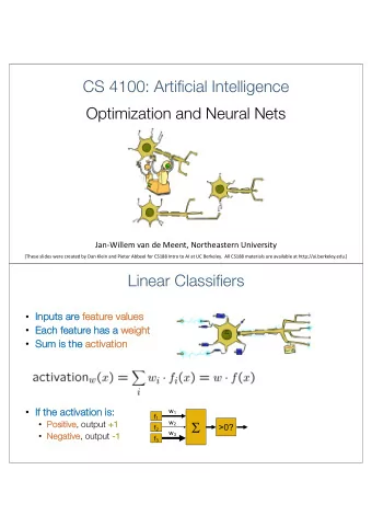
Reminder: Linear Classifiers  Inputs are feature values  Each feature has a weight  Sum is the activation  If the activation is: w 1 f 1   Positive, output +1 w 2 >0? f 2 w 3  Negative, output -1 f 3

How to get probabilistic decisions?  Activation:  If very positive  want probability going to 1  If very negative  want probability going to 0  Sigmoid function

Best w?  Maximum likelihood estimation: with: = Logistic Regression

Multiclass Logistic Regression  Multi-class linear classification  A weight vector for each class:  Score (activation) of a class y:  Prediction w/highest score wins:  How to make the scores into probabilities? original activations softmax activations

Best w?  Maximum likelihood estimation: with: = Multi-Class Logistic Regression

This Lecture  Optimization  i.e., how do we solve:

Hill Climbing  Recall from CSPs lecture: simple, general idea  Start wherever  Repeat: move to the best neighboring state  If no neighbors better than current, quit  What’s particularly tricky when hill -climbing for multiclass logistic regression? • Optimization over a continuous space • Infinitely many neighbors! • How to do this efficiently?

1-D Optimization  Could evaluate and  Then step in best direction  Or, evaluate derivative:  Tells which direction to step into

2-D Optimization Source: offconvex.org

Gradient Ascent  Perform update in uphill direction for each coordinate  The steeper the slope (i.e. the higher the derivative) the bigger the step for that coordinate  E.g., consider:  Updates:  Updates in vector notation: with: = gradient

Gradient Ascent  Idea:  Start somewhere  Repeat: Take a step in the gradient direction Figure source: Mathworks

What is the Steepest Direction?  First-Order Taylor Expansion:  Steepest Descent Direction:  Recall:   Hence, solution: Gradient direction = steepest direction!

Gradient in n dimensions

Optimization Procedure: Gradient Ascent  init  for iter = 1, 2, …  : learning rate --- tweaking parameter that needs to be chosen carefully  How? Try multiple choices  Crude rule of thumb: update changes about 0.1 – 1 %

Batch Gradient Ascent on the Log Likelihood Objective  init  for iter = 1, 2, …

Stochastic Gradient Ascent on the Log Likelihood Objective Observation: once gradient on one training example has been computed, might as well incorporate before computing next one  init  for iter = 1, 2, …  pick random j

Mini-Batch Gradient Ascent on the Log Likelihood Objective Observation: gradient over small set of training examples (=mini-batch) can be computed in parallel, might as well do that instead of a single one  init  for iter = 1, 2, …  pick random subset of training examples J

How about computing all the derivatives?  We’ll talk about that once we covered neural networks, which are a generalization of logistic regression

Neural Networks

Multi-class Logistic Regression  = special case of neural network f 1 (x) s z 1 o f 2 (x) f t z 2 m f 3 (x) a x … z 3 f K (x)

Deep Neural Network = Also learn the features! f 1 (x) s z 1 o f 2 (x) f t z 2 m f 3 (x) a x … z 3 f K (x)

Deep Neural Network = Also learn the features! x 1 f 1 (x) s o x 2 f 2 (x) f … t x 3 m f 3 (x) a x … … … … … x L f K (x) g = nonlinear activation function

Deep Neural Network = Also learn the features! x 1 s o x 2 f … t x 3 m a x … … … … … x L g = nonlinear activation function

Common Activation Functions [source: MIT 6.S191 introtodeeplearning.com]

Deep Neural Network: Also Learn the Features!  Training the deep neural network is just like logistic regression: just w tends to be a much, much larger vector   just run gradient ascent + stop when log likelihood of hold-out data starts to decrease

Neural Networks Properties  Theorem (Universal Function Approximators). A two-layer neural network with a sufficient number of neurons can approximate any continuous function to any desired accuracy.  Practical considerations  Can be seen as learning the features  Large number of neurons  Danger for overfitting  (hence early stopping!)

Universal Function Approximation Theorem*  In words: Given any continuous function f(x), if a 2-layer neural network has enough hidden units, then there is a choice of weights that allow it to closely approximate f(x). Cybenko (1989) “Approximations by superpositions of sigmoidal functions” Hornik (1991) “Approximation Capabilities of Multilayer Feedforward Networks” Leshno and Schocken (1991) ”Multilayer Feedforward Networks with Non -Polynomial Activation Functions Can Approximate Any Function”

Universal Function Approximation Theorem* Cybenko (1989) “Approximations by superpositions of sigmoidal functions” Hornik (1991) “Approximation Capabilities of Multilayer Feedforward Networks” Leshno and Schocken (1991) ”Multilayer Feedforward Networks with Non -Polynomial Activation Functions Can Approximate Any Function”

Fun Neural Net Demo Site  Demo-site:  http://playground.tensorflow.org/

How about computing all the derivatives?  Derivatives tables: [source: http://hyperphysics.phy-astr.gsu.edu/hbase/Math/derfunc.html

How about computing all the derivatives?  But neural net f is never one of those?  No problem: CHAIN RULE: If Then  Derivatives can be computed by following well-defined procedures

Automatic Differentiation  Automatic differentiation software  e.g. Theano, TensorFlow, PyTorch, Chainer  Only need to program the function g(x,y,w)  Can automatically compute all derivatives w.r.t. all entries in w  This is typically done by caching info during forward computation pass of f, and then doing a backward pass = “backpropagation”  Autodiff / Backpropagation can often be done at computational cost comparable to the forward pass  Need to know this exists  How this is done? -- outside of scope of CS188

Summary of Key Ideas  Optimize probability of label given input  Continuous optimization  Gradient ascent:  Compute steepest uphill direction = gradient (= just vector of partial derivatives)  Take step in the gradient direction  Repeat (until held- out data accuracy starts to drop = “early stopping”)  Deep neural nets  Last layer = still logistic regression  Now also many more layers before this last layer  = computing the features   the features are learned rather than hand-designed  Universal function approximation theorem  If neural net is large enough  Then neural net can represent any continuous mapping from input to output with arbitrary accuracy  But remember: need to avoid overfitting / memorizing the training data  early stopping!  Automatic differentiation gives the derivatives efficiently (how? = outside of scope of 188)

How well does it work?