Algorithms: Gradient Descent This classic greedy algorithm for - - PowerPoint PPT Presentation

SLIDE 1

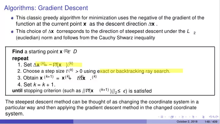
Algorithms: Gradient Descent

This classic greedy algorithm for minimization uses the negative of the gradient of the

function at the current point x as the descent direction ∆x .

∗ ∗

This choice of ∆x corresponds to the direction of steepest descent under the L

∗ 2

(eucledian) norm and follows from the Cauchy Shwarz inequality

Find a starting point x ∈ D

(0)

repeat

• 1. Set ∆x

= −∇f(x ).

(k) (k)

• 2. Choose a step size t (k) > 0 using exact or backtracking ray search.
• 3. Obtain x (k+1) =

+ ∆x .

x(k)

t(k)

(k)

• 4. Set k = k + 1.

until stopping criterion (such as ||∇f(x

(k+1) )|| ≤ ϵ) is satisfed

2

The steepest descent method can be thought of as changing the coordinate system in a particular way and then applying the gradient descent method in the changed coordinate

system.

October 2, 2018 148 / 409

SLIDE 2

Convergence of the Gradient Descent Algorithm

We recap the (necessary) inequality (36) resulting from Lipschitz continuity of ∇f(x): f(y) ≤ f(x) + ∇ f(x)(y − x) +

⊤ L

2

∥y − x∥

2

Considering x ≡ x, and x = x − t ∇f(x ) ≡ y, we get

k k+1 k k k

October 2, 2018 149 / 409

SLIDE 3

Convergence of the Gradient Descent Algorithm

We recap the (necessary) inequality (36) resulting from Lipschitz continuity of ∇f(x): f(y) ≤ f(x) + ∇ f(x)(y − x) +

⊤ L

2

∥y − x∥

2

Considering x ≡ x, and x = x − t ∇f(x ) ≡ y, we get

k k+1 k k k

f(x k+1 ) ≤ f(x ) − t ∇ f(x )∇f(x ) +

k k ⊤ k k

L t ( )

k

2

2

∇f(x )

k 2

=⇒ f(x k+1 ) ≤ f(x ) − (1 −

k

Ltk

2

)t∇f(x )

k 2

We desire to have the following (46). It holds if.... f(x k+1 ) ≤ f(x ) −

k

b

t

2

∇f(x )

k 2

(46)

October 2, 2018 149 / 409

SLIDE 4

Convergence of the Gradient Descent Algorithm

We recap the (necessary) inequality (36) resulting from Lipschitz continuity of ∇f(x): f(y) ≤ f(x) + ∇ f(x)(y − x) +

⊤ L

2

∥y − x∥

2

Considering x ≡ x, and x = x − t ∇f(x ) ≡ y, we get

k k+1 k k k

f(x k+1 ) ≤ f(x ) − t ∇ f(x )∇f(x ) +

k k ⊤ k k

L t ( )

k

2

2

∇f(x )

k 2

=⇒ f(x k+1 ) ≤ f(x ) − (1 −

k

Ltk

2

)t∇f(x )

k 2

We desire to have the following (46). It holds if.... f(x k+1 ) ≤ f(x ) −

k

b

t

2

∇f(x )

k 2

(46)

▶ With fxed step size t = b k

t, we ensure that 0 < bt ≤

1

L

=⇒ 1 −

b

Lt 2 ≥ 1 2.

▶ With backtracking step seach, (46) holds with b

t = min 1, β {

2(1−

1) c

L

}

See https://www.youtube.com/watch?v=SGZdsQviFYs&list=PLsd82ngobrvcYfCdnSnqM7lKLqE9qUUpX&index=17 October 2, 2018 149 / 409

the drop in the value of the objective will be atleast order of

square of norm

• f gradient

derivation provided a few slides later

SLIDE 5

Aside: Backtracking ray search and Lipschitz Continuity

Recap the Backtracking ray search algorithm

▶ Choose a β ∈ (0, 1) ▶ Start with t = 1 ▶ While f(x + t∆x) > f(x) + c t∇ f(x)∆x, do

1 T

⋆ Update t ← βt

On convergence, f(x + t∆x) ≤ f(x) + c t∇ f(x)∆x

1

T

For gradient descent, this means f(x + t∆x) ≤ f(x) − c t∥∇f(x)∥

1 2

For a function f with Lipschitz continuous ∇f(x) we have that f(x k+1 ) ≤ f(x k) − b

t

2

∇f(x ) is satisfed if b

k

2

t = min 1, β {

2(1− 1)

c

L

}

Reason: With backtracking step seach, if 1 −

Lt k

2 ≥ c , the Armijo rule will be satisfed. 1

That is, 0 < t ≤

k 2(1− 1)

c

L

=⇒ 1 −

Lt k

2 ≥ c . If not, there must exist an interger j for 1

which β 2(1− 1)

c

L

≤ β ≤

j

2(1−c 1) L

, we take b

t = min 1, β {

2(1− 1)

c

L

}

October 2, 2018 152 / 409

SLIDE 6

Using convexity, we have f(x ) ≥ f(x ) + ∇ f(x )(x − x )

∗

k ⊤ k

∗

k

=⇒ f(x ) ≤ f(x ) + ∇ f(x )(x − x )

k

∗

⊤ k k

∗

Thus, f(x k+1 ) ≤ f(x ) −

k t

2

∇f(x )

k 2

=⇒ f(x k+1 ) ≤ f(x ) + ∇ f(x )(x − x ) −

∗

⊤ k k

∗

t

2

∇f(x )

k 2

=⇒ f(x k+1 ) ≤ f(x )+

∗ 1

2t k

x − x +∇ f(x )(x − x ) −

∗

2 T k k

∗

t

2

∇f(x ) −

k 2

1

2t k

x − x

∗

2

October 2, 2018 150 / 409

SLIDE 7

Using convexity, we have f(x ) ≥ f(x ) + ∇ f(x )(x − x )

∗

k ⊤ k

∗

k

=⇒ f(x ) ≤ f(x ) + ∇ f(x )(x − x )

k

∗

⊤ k k

∗

Thus, f(x k+1 ) ≤ f(x ) −

k t

2

∇f(x )

k 2

=⇒ f(x k+1 ) ≤ f(x ) + ∇ f(x )(x − x ) −

∗

⊤ k k

∗

t

2

∇f(x )

k 2

=⇒ f(x k+1 ) ≤ f(x )+

∗ 1

2t k

x − x +∇ f(x )(x − x ) −

∗

2 T k k

∗

t

2

∇f(x ) −

k 2

1

2t k

x − x

∗

2

=⇒ f(x k+1 ) ≤ f(x ) +

∗ 1

2t

(x − x −x − x − t∇f(x ) )

k

∗

2 k

∗

k 2

=⇒ f(x k+1 ) ≤ f(x ∗) +

1

2t

(x − x −x

k

∗

2 k+1

− x )

∗

2

=⇒ f(x k+1 ) − f(x ) ≤

∗

1

2t

(x − x −x

k

∗

2 k+1

− x )

∗

2

(47)

October 2, 2018 150 / 409

SLIDE 8

∗

∑ (

i=1

f(x ) − f(x ) ≤

i ∗

)

1

2t

( x

(0) − x∗ ) 2

)

The ray and line search ensure that f(x

6

i+1 ) ≤ f(x ) ∀i = 0, 1, . . . , k. We thus get

i

6By Armijo condition in (29), for some 0 < c1 < 1, f(x

i+1 ) ≤ f(x ) + c1t ∇ f(x )∆x i i T i i October 2, 2018 151 / 409

SLIDE 9

∗

∑ (

i=1

f(x ) − f(x ) ≤

i ∗

)

1

2t

( x

(0) − x∗ ) 2

)

The ray and line search ensure that f(x

6

i+1 ) ≤ f(x ) ∀i = 0, 1, . . . , k. We thus get

i

f(x ) − f(x ) ≤

k

∗

1

k

k (

∑

i=1

f(x ) − f(x ) ≤

i ∗

) x

(0) − x∗ 2

2tk Thus, as k → ∞, f(x ) → f(x ). This shows convergence for gradient descent.

k

∗

6By Armijo condition in (29), for some 0 < c1 < 1, f(x

i+1 ) ≤ f(x ) + c1t ∇ f(x )∆x i i T i i October 2, 2018 151 / 409

To get epsilon close to f(x*), it is sufficient for k to be O(1/epsilon)

SLIDE 10

Rates of Convergence

October 2, 2018 153 / 409

SLIDE 11

Convergence

October 2, 2018 154 / 409

• bserve acceleration

(this is what we observed for the better algo for Rosenbrack function) rate of convergence = slope increasing

• rder

SLIDE 12

Linear Convergence

v , . . . , v is Linearly (or specifcally, Q-linearly) convergent if

1

k k+1

v

− v

∗

v − v

k

∗

≤ r

for some k ≥ θ, and r ∈ (0, 1)

▶ ‘Q’ here stands for ‘quotient’ of the norms as shown above

October 2, 2018 155 / 409

SLIDE 13

Q-convergence

v , . . . , v is Q-linearly convergent if

1

k k+1

v

− v

∗

v − v

k

∗

≤ r

for some k ≥ θ, and r ∈ (0, 1)

▶ ‘Q’ here stands for ‘quotient’ of the norms as shown above ▶ Consider the sequence s s =

1 1

[ 11

2 , 21 4 , 41 8 , . . . , 5 + 1 2

n , . . .]

The sequence converges to

October 2, 2018 156 / 409

5

SLIDE 14

Q-convergence

v , . . . , v is Q-linearly convergent if

1

k k+1

v

− v

∗

v − v

k

∗

≤ r

for some k ≥ θ, and r ∈ (0, 1)

▶ ‘Q’ here stands for ‘quotient’ of the norms as shown above ▶ Consider the sequence s s =

1 1

[ 11

2 , 21 4 , 41 8 , . . . , 5 + 1 2

n , . . .]

The sequence converges to s = 5 and it is

∗ 1

October 2, 2018 156 / 409

Q-linearly convergent

SLIDE 15

Q-convergence

v , . . . , v is Q-linearly convergent if

1

k k+1

v

− v

∗

v − v

k

∗

≤ r

for some k ≥ θ, and r ∈ (0, 1)

▶ ‘Q’ here stands for ‘quotient’ of the norms as shown above ▶ Consider the sequence s s =

1 1

[ 11

2 , 21 4 , 41 8 , . . . , 5 + 1 2

n , . . .]

The sequence converges to s = 5 and it is Q-linear convergence because:

∗ 1 k+1

s

1

− s

∗ 1

s − s

k

1 ∗ 1

=

1 1 2

k+1

1 2

k =

1 2 < 0.6(= M)

▶ How about the convergence result we got by assuming Lipschitz continuity with backtracking

and exact line searches?

October 2, 2018 156 / 409

SLIDE 16

Generalizing Q-convergence to R-convergence

Consider the sequence r r = 5,

1 1 21 4 , 21 4 , . . . , 5 + 1 4

⌊

n

2 ⌋ , . . .

The sequence converges to

October 2, 2018 157 / 409

5

SLIDE 17

Generalizing Q-convergence to R-convergence

Consider the sequence r r = 5,

1 1 21 4 , 21 4 , . . . , 5 + 1 4

⌊

n

2 ⌋ , . . .

The sequence converges to s = 5 but not Q-linearly!

∗ 1

Let us consider the convergence result we got by assuming Lipschitz continuity with

backtracking and exact line searches:

f(x ) − f(x ) ≤

k

∗

x − x

(0)

∗

2

2tk

October 2, 2018 157 / 409

SLIDE 18

Generalizing Q-convergence to R-convergence

Consider the sequence r r = 5,

1 1 21 4 , 21 4 , . . . , 5 + 1 4

⌊

n

2 ⌋ , . . .

The sequence converges to s = 5 but not Q-linearly!

∗ 1

Let us consider the convergence result we got by assuming Lipschitz continuity with

backtracking and exact line searches:

f(x ) − f(x ) ≤

k

∗

x − x

(0)

∗

2

2tk Q-convergence by itself insufcient. We will generalize it to R-convergence. ‘R’ here stands for ‘root’, as we are looking at convergence rooted at x ∗ We say that the sequence s , . . . , s is R-linearly convergent if s − s ≤ v , ∀k, and

1

k k

∗

k

{ }

vk converges Q-linearly to zero

October 2, 2018 157 / 409

SLIDE 19

R-convergence assuming Lipschitz continuity

Consider v =

k

∥x (0) − x ∥

∗

2

2tk

=

α k , where α is a constant

Here, we have ∥vk+1

−v ∥ ∗

∥v −v ∥

k

∗ October 2, 2018 158 / 409

<= k/(k+1) --> 1 as k tends to infinity

SLIDE 20

R-convergence assuming Lipschitz continuity

Consider v =

k

∥x (0) − x ∥

∗

2

2tk

=

α k , where α is a constant

Here, we have ∥vk+1

−v ∥ ∗

∥v −v ∥

k

∗

≤

K K+1 , where K is the fnal number of iterations

▶

K K+1 < 1, but we don’t have K K+1 < r

Thus, v =

k α k is not Q-linearly convergent as there exist no v < 1 s.t. α/(k+1) α/k

=

k k+1 ≤ v, ∀k ≥ θ

Strictly speaking, for Lipschitz continuity alone, gradient descent is not guaranteed to

give R-linear convergence

In practice, Lipschitz continuity gives “almost” R-linear convergence – not too bad! We say that gradient descent with Lipschtiz continuity has convergence rate O(1/k), that

is,

October 2, 2018 158 / 409

SLIDE 21

R-convergence assuming Lipschitz continuity

Consider v =

k

∥x (0) − x ∥

∗

2

2tk

=

α k , where α is a constant

Here, we have ∥vk+1

−v ∥ ∗

∥v −v ∥

k

∗

≤

K K+1 , where K is the fnal number of iterations

▶

K K+1 < 1, but we don’t have K K+1 < r

Thus, v =

k α k is not Q-linearly convergent as there exist no v < 1 s.t. α/(k+1) α/k

=

k k+1 ≤ v, ∀k ≥ θ

Strictly speaking, for Lipschitz continuity alone, gradient descent is not guaranteed to

give R-linear convergence

In practice, Lipschitz continuity gives “almost” R-linear convergence – not too bad! We say that gradient descent with Lipschtiz continuity has convergence rate O(1/k), that is, to obtain f(x ) − f(x ) ≤ ϵ, we need O(

k

∗ 1 ϵ ) iterations.

October 2, 2018 158 / 409

SLIDE 22

Taking hint from this analysis, if Q-linear,

s − s

∗

s − s

k

∗

≤ r

∈ (0, 1)

then,

k+1

s − s ≤ rs − s

∗

k

∗

≤ r s

2

k −1

− s

∗

. . .

≤ r s − s , which is v for R-linear

k (0)

∗

k

Thus, Q-linear convergence =⇒ R-linear convergence

▶ Q-linear is a special case of R-linear

▶ R-linear gives a more general way of characterizing linear convergence

Q-linear is an ‘order of convergence’

r is the ‘rate of convergence’

October 2, 2018 159 / 409

Any Q-linearly convergent sequence is also R-linearly convergent

SLIDE 23

Question: Could we analyze Gradient descent more specifcally? Assume backtracking line search

Continue assuming Lipschitz continuity

▶ Curvature is upper bounded: ∇ f(x) ⪯ LI

2

Assume strong convexity

▶ Curvature is lower bounded: ∇ f(x) ⪰ mI

2

▶ For instance, we might not want to use gradient descent for a quadratic function (curvature

is not accounted for)

October 2, 2018 163 / 409

Could we either look at more conditions (strong convexity) for better order of convergence for existing gradient descent? Could we either look at completely different algorithms for better order of convergence? Without strong convexity grad descent = R sublinear With strong convexity, grad descent also Q linear

SLIDE 24

There exits (Fenchel) duality between strong convexity and Lipschitz continuous gradient. That is, with a good understanding of one, we can easily understand the other one. See

http://xingyuzhou.org/talks/Fenchel_duality.pdf for a quick summary!

(Better) Convergence Using Strong Convexity

October 2, 2018 164 / 409

SLIDE 25

Proof of Second Order Conditions for Convexity

In other words ∇ f(x) ⪰ cIn×n

2

where In×n is the n × n identity matrix and ⪰ corresponds to the positive semidefnite

• inequality. That is, the function f is strongly convex if ∇ f(x) − cIn×n is positive semidefnite,

2

for all x ∈ D and for some constant c > 0, which corresponds to the positive minimum

curvature of f. PROOF: We will prove only the frst statement; the other two statements are proved in a similar manner.

Necessity: Suppose f is a convex function, and consider a point x ∈ D. We will prove that for any h ∈ ℜ , h ∇ f(x)h ≥ 0. Since f is convex, we have

n

T

2

f(x + th) ≥ f(x) + t∇ f(x)h

T

(48) Consider the function ϕ(t) = f(x + th) defned on the domain D = [0, 1].

ϕ

October 2, 2018 166 / 409

SLIDE 26

Lipschitz Continuity vs. Strong Convexity

Lipschitz continuity of gradient (references to ∇ assume double diferentiability)

2

∇ f(x) ⪯ LI

∇f(x) − ∇f(y) ≤ L∥x − y∥

2

f(y) ≤ f(x) + ∇ f(x)(y − x) +

⊤

L

2

∥y − x∥ 2

Strong convexity: Curvature should be atleast somewhat positive

∇ f(x) ⪰ mI

2

f(y) ≥ f(x) + ∇ f(x)(y − x) +

⊤

m

2

∥y − x∥ 2

▶ m = 0 corresponds to (sufcient condition for) normal convexity.

▶ Later: For example, augmented Lagrangian is used to introduce strong convexity

October 2, 2018 170 / 409