LOGISTIC REGRESSION, GRADIENT LOGISTIC REGRESSION, GRADIENT - PowerPoint PPT Presentation

LOGISTIC REGRESSION, GRADIENT LOGISTIC REGRESSION, GRADIENT DESCENT, NEWTON DESCENT, NEWTON Matthieu R Bloch Thursday, January 30, 2020 1

LOGISTICS LOGISTICS TAs and Office hours Monday: Mehrdad (TSRB 523a) - 2pm-3:15pm Tuesday: TJ (VL C449 Cubicle D) - 1:30pm - 2:45pm Wednesday: Matthieu (TSRB 423) - 12:00:pm-1:15pm Thursday: Hossein (VL C449 Cubicle B): 10:45pm - 12:00pm Friday: Brighton (TSRB 523a) - 12pm-1:15pm Homework 1 Hard deadline Friday January 31, 2020 (11:59PM EST) (Wednesday February 5, 2020 for DL) Homework 2 posted Due Wednesday February7,2020 11:59pm EST(Wednesday February14, 2020 for DL) 2

RECAP: GENERATIVE MODELS RECAP: GENERATIVE MODELS Quadratic Discriminant Analysis: classes distributed according to N ( μ k Σ k , ) Covariance matrices are class dependent but decision boundary not linear anymore Generative model rarely accurate Number of parameters to estimate: class priors, means, elements of covariance matrix 1 K − 1 Kd d ( d + 1) Works well if 2 N ≫ d Works poorly if without other tricks (dimensionality reduction, structured covariance) N ≪ d Biggest concern: “one should solve the [classification] problem directly and never solve a more general problem as an intermediate step [such as modeling p(xly)].” , Vapnik, 1998 Revisit binary classifier with LDA π 1 ϕ ( x ; μ 1 , Σ) 1 η 1 ( x ) = = w ⊺ π 1 ϕ ( x ; μ 1 , Σ) + π 0 ϕ ( x ; μ 0 , Σ) 1 + exp(−( x + b )) We no not need to estimate the full joint distribution! 3

4

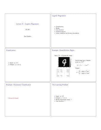
LOGISTIC REGRESSION LOGISTIC REGRESSION Assume that is of the form 1 η ( x ) w ⊺ 1+exp(−( x + b )) Estimate and from the data directly ^ w ^ b Plugin the result to obtain 1 η ^ ( x ) = ^ ⊺ ^ 1+exp(−( x + )) w b The function is called the logistic function 1 x ↦ 1+ e − x The binary logistic classifier is ( linear ) 1 ^ ⊺ h LC ^ ( x ) = 1 { ( x ) ≥ η } = 1 { w x + b ≥ 0} ^ 2 How do we estimate and ? ^ w b ^ From LDA analysis: , ^ −1 μ ^ −1 μ ^ −1 μ ^ ⊺ ^ ⊺ π ^ 1 1 1 w = Σ ( − μ ) b = 2 μ 0 Σ − 2 μ 1 Σ + log ^ ^ 1 ^ 0 ^ 0 ^ 1 π ^ 0 Direct estimation of from maximum likelihood ( w , b ) ^ 5

MLE FOR LOGISTIC REGRESSION MLE FOR LOGISTIC REGRESSION We have a parametric density model for p θ ( y | x ) = η ^ ( x ) Standard trick: and x ⊺ ] ⊺ θ = [ b w ⊺ ] ⊺ ~ x = [1, This allows us to lump the offset and write 1 η ( x ) = θ ⊺ x ~ 1 + exp(− ) Given our dataset the likelihood is ∏ N ~ i y i } N ~ i {( x , ) L ( θ ) ≜ i =1 P θ y i x ( | ) i =1 For with we obtain K = 2 Y = {0, 1} N ~ i ) y i ~ i ) 1− y i L ( θ ) ≜ ∏ η ( x (1 − η ( x ) i =1 N ~ i ~ i ℓ( θ ) = ∑ ( y i log η ( x ) + (1 − y i ) log(1 − η ( x ))) i =1 N e θ ⊺ x ~ i y i θ ⊺ x ~ i ℓ( θ ) = ∑ ( − log(1 + ) ) i =1 6

7

8

FINDING THE MLE FINDING THE MLE A necessary condition for optimality is ∇ θ ℓ( θ ) = 0 Here this means ∑ N 1 ~ i i =1 x ( y i − ) = 0 θ ⊺ x ~ i 1+exp(− ) System of non linear equations! d + 1 Use numerical algorithm to find the solution of argmin θ − ℓ( θ ) Provable convergence when is convex −ℓ We will discuss two techniques: Gradient descent Newton’s method There are many more, especially useful in high dimension 9

WRAPPING UP PLUGIN METHODS WRAPPING UP PLUGIN METHODS Naive Bayes, LDA, and logistic regression are all plugin methods that result in linear classifiers Naive Bayes plugin method based on density estimation scales well to high-dimensions and naturally handles mixture of discrete and continuous features Linear discriminant analysis better if Gaussianity assumptions are valid Logistic regression models only the distribution of , not P y | x P y , x valid for a larger class of distributions fewer parameters to estimate Plugin methods can be useful in practice, but ultimately they are very limited There are always distributions where our assumptions are violated If our assumptions are wrong, the output is totally unpredictable Can be hard to verify whether our assumptions are right Require solving a more difficult problem as an intermediate step 10

GRADIENT DESCENT GRADIENT DESCENT Consider the canonical problem R d min f ( x ) with f : → R x ∈ R d Find minimum by find iteratively by “rolling downhill” Start from point x (0) ; is the step size x (1) x (0) = − η ∇ f ( x ) | x = x (0) η x (2) x (1) = − η ∇ f ( x ) | x = x (1) ⋯ Choice of step size really matters: too small and convergence takes forever, too big and might η never converge Many variants of gradient descent Momentum: and x ( t +1) x ( t ) v t = γ v t −1 + η ∇ f ( x ) | x = x ( t ) = − v t Accelerated: and x ( t +1) x ( t ) v t = γ v t −1 + η ∇ f ( x ) | x = = − v t x ( t ) − γ v t −1 In practice, gradient has to be evaluated from data 11

NEWTON’S METHOD NEWTON’S METHOD Newton-Raphson method uses the second derivative to automatically adapt step size x ( j +1) x ( j ) ∇ 2 ] −1 = − [ f ( x ) ∇ f ( x ) | x = x j Hessian matrix ∂ 2 ∂ 2 ∂ 2 f f f ⋯ ⎡ ⎤ ∂ x 2 ∂ x 1 x 2 ∂ ∂ x 1 x d ∂ 1 ⎢ ⎥ ∂ 2 ∂ 2 ∂ 2 ⎢ f f f ⎥ ⋯ ⎢ ⎥ ∂ x 2 ∂ x 1 x 2 ∂ ∂ x 2 x d ∂ ⎢ ⎥ ∇ 2 2 f ( x ) = ⎢ ⎥ ⎢ ⎥ ⎢ ⎥ ⋮ ⋮ ⋱ ⋮ ⎢ ⎥ ⎢ ⎥ ∂ 2 ∂ 2 ∂ 2 f f f ⎣ ⋯ ⎦ ∂ x 2 ∂ x d x 1 ∂ ∂ x d x 2 ∂ d Newton’s method is much faster when the dimension is small but impractical when is large d d 12

STOCHASTIC GRADIENT DESCENT STOCHASTIC GRADIENT DESCENT O�en have a loss function of the form where ∑ N ℓ( θ ) = i =1 ℓ i ( θ ) ℓ i ( θ ) = f ( x i y i , , θ ) The gradient is and gradient descent update is ∑ N ∇ θ ℓ( θ ) = ∇ ( θ ) ℓ i i =1 N θ ( j +1) θ ( j ) = − η ∑ ∇ ( θ ) ℓ i i =1 Problematic if dataset if huge of if not all data is availabel Use iterative technique instead θ ( j +1) θ ( j ) = − η ∇ ( θ ) ℓ i Tons of variations of principle Batch, minibatch, Adagrad, RMSprop, Adam, etc. 13

   14