Logistic regression Shay Cohen (based on slides by Sharon - PowerPoint PPT Presentation
Logistic regression Shay Cohen (based on slides by Sharon Goldwater) 28 October 2019 Todays lecture How can we use logistic regression for reranking? How do we set the parameters of a logistic regression model? How is logistic
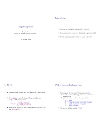
Logistic regression Shay Cohen (based on slides by Sharon Goldwater) 28 October 2019
Today’s lecture ◮ How can we use logistic regression for reranking? ◮ How do we set the parameters of a logistic regression model? ◮ How is logistic regression related to neural networks?
The Model ◮ Decide on some features that associate certain � x with certain y ◮ Uses exp( z ) to make all values of dot-product between weights and features positive exp( � i w i f i ( � x , y )) P ( y | � x ) = � y ′ exp( � i w i f i ( � x , y ′ )) ◮ We divide by the sum of all exp-dot-product values for all y so that sum y p ( y | � x ) = 1
WSD as example classification task ◮ Disambiguate three senses of the target word plant ◮ � x are the words and POS tags in the document the target word occurs in ◮ y is the latent sense. Assume three possibilities: y = sense 1 Noun: a member of the plant kingdom 2 Verb: to place in the ground 3 Noun: a factory ◮ We want to build a model of P ( y | � x ).
Defining a MaxEnt model: intuition ◮ Start by defining a set of features that we think are likely to help discriminate the classes. E.g., ◮ the POS of the target word ◮ the words immediately preceding and following it ◮ other words that occur in the document ◮ During training, the model will learn how much each feature contributes to the final decision.
MaxEnt for n-best re-ranking ◮ So far, we’ve used logistic regression for classification . ◮ Fixed set of classes, same for all inputs. ◮ Word sense disambiguation: Input Possible outputs word in doc1 sense 1, sense 2, sense 3 word in doc2 sense 1, sense 2, sense 3 ◮ Dependency parsing: Input Possible outputs parser config1 action 1, . . . action n parser config2 action 1, . . . action n
MaxEnt for n-best re-ranking ◮ We can also use MaxEnt for reranking an n -best list. ◮ Example scenario (Charniak and Johnson, 2005) ◮ Use a generative parsing model M with beam search to produce a list of the top n parses for each sentence. (= most probable according to M ) ◮ Use a MaxEnt model M ′ to re-rank those n parses, then pick the most probable according to M ′ .
Why do it this way? Why two stages? ◮ Generative models typically faster to train and run, but can’t use arbitrary features. ◮ In NLP, MaxEnt models may have so many features that extracting them from each example can be time-consuming, and training is even worse (see next lecture). Why are the features a function of both inputs and outputs? ◮ Because for re-ranking this matters: the outputs may not be pre-defined.
MaxEnt for n-best re-ranking ◮ In reranking scenario, the options depend on the input . E.g., parsing, with n = 2: ◮ Input: healthy dogs and cats ◮ Possible outputs: NP NP JJ NP NP CC NP healthy NP CC NP JJ NP and cats dogs and cats healthy dogs
MaxEnt for n-best re-ranking ◮ In reranking scenario, the options depend on the input . E.g., parsing, with n = 2: ◮ Input: ate pizza with cheese ◮ Possible outputs: VP VP V NP VP PP ate V NP P NP NP PP ate pizza with cheese pizza P NP with cheese
MaxEnt for constituency parsing ◮ Now we have y = parse tree, x = sentence. ◮ Features can mirror parent-annotated/lexicalized PCFG: ◮ counts of each CFG rule used in y ◮ pairs of words in head-head dependency relations in y ◮ each word in x with its parent and grandparent categories in y . ◮ Note these are no longer binary features.
Global features ◮ Features can also capture global structure. E.g., from Charniak and Johnson (2005): ◮ length difference of coordinated conjuncts NP vs NP JJ NP NP CC NP healthy NP CC NP JJ NP and cats dogs and cats healthy dogs
Features for parsing ◮ Altogether, Charniak and Johnson (2005) use 13 feature templates ◮ with a total of 1,148,697 features ◮ and that is after removing features occurring less than five times ◮ One important feature not mentioned earlier: the log prob of the parse under the generative model! ◮ So, how does it do?
Parser performance ◮ F 1 -measure (from precision/recall on constituents) on WSJ test: ∼ 80% 1 standard PCFG lexicalized PCFG (Charniak, 2000) 89.7% re-ranked LPCFG (Charniak and Johnson, 2005) 91.0% 1 Figure from Charniak (1996): assumes POS tags as input
Parser performance ◮ F 1 -measure (from precision/recall on constituents) on WSJ test: ∼ 80% 1 standard PCFG lexicalized PCFG (Charniak, 2000) 89.7% re-ranked LPCFG (Charniak and Johnson, 2005) 91.0% ◮ Recent WSJ parser is 93.8%, combining NNets and ideas from parsing, language modelling (Choe et al., 2016) ◮ But as discussed earlier, other languages/domains are still much worse.
Evaluating during development Whenever we have a multistep system, worth asking: where should I put my effort to improve the system? ◮ If my first stage (generative model) is terrible, then n needs to be very large to ensure it includes the correct parse. ◮ Worst case: if computation is limited ( n is small), maybe the correct parse isn’t there at all. ◮ Then it doesn’t matter how good my second stage is, I won’t get the right answer.
Another use of oracles Can be useful to compute oracle performance on the first stage. ◮ Oracle always chooses the correct parse if it is available. ◮ Difference between oracle and real system = how much better it could get by improving the 2nd stage model. ◮ If oracle performance is very low, need to increase n or improve the first stage model.
How do we use the weights in practice? A question asked in a previous class. The following (over-)simplification chooses the best y according to the model (in the case of a small set of labels). Given an x : ◮ For each y , calculate f i ( � x , y ) for all y and i ◮ For each y , calculate � i w i f i ( � x , y ) ◮ Choose the y with the highest score: y ∗ = arg max y � i w i f i ( � x , y )
Training the model Two ways to think about training: ◮ What is the goal of training ( training objective )? ◮ How do we achieve that goal (training algorithm)?
Training generative models ◮ Easy to think in terms of how : counts/smoothing. ◮ But don’t forget the what : What How Maximize the likelihood take raw counts and normalize Other objectives 1 use smoothed counts 1 Historically, smoothing methods were originally introduced purely as how : that is, without any particular justification as optimizing some objective function. However, as alluded to earlier, it was later discovered that many of these smoothing methods correspond to optimizing Bayesian objectives. So the what was discovered after the how .
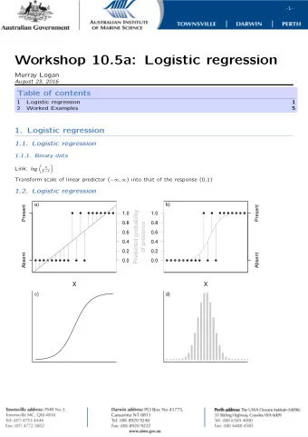
Training logistic regression Possible training objective: ◮ Given annotated data, choose weights that make the labels most probable under the model. ◮ That is, given items x (1) . . . x ( N ) with labels y (1) . . . y ( N ) , choose � log P ( y ( j ) | x ( j ) ) w = argmax ˆ w � j ◮ This is conditional maximum likelihood estimation (CMLE).
Regularization ◮ Like MLE for generative models, CMLE can overfit training data. ◮ For example, if some particular feature combination is only active for a single training example. ◮ So, add a regularization term to the equation ◮ encourages weights closer to 0 unless lots of evidence otherwise. ◮ various methods; see JM3 or ML texts for details (optional). ◮ In practice it may require some experimentation (dev set!) to choose which method and how strongly to penalize large weights.
Optimizing (regularized) cond. likelihood ◮ Unlike generative models, we can’t simply count and normalize. ◮ Instead, we use gradient-based methods, which iteratively update the weights. ◮ Our objective is a function whose value depends on the weights. ◮ So, compute the gradient (derivative) of the function with respect to the weights. ◮ Update the weights to move toward the optimum of the objective function.
Visual intuition ◮ Changing � w changes the value of the objective function. 2 ◮ Follow the gradients to optimize the objective (“hill-climbing”). 2 Here, we are maximizing an objective such as log prob. Using an objective such as negative log prob would require minimizing ; in this case the objective function is also called a loss function .
But what if...? ◮ If there are multiple local optima , we won’t be guaranteed to find the global optimum .
Guarantees ◮ Luckily, (supervised) logistic regression does not have this problem. ◮ With or without standard regularization, the objective has a single global optimum. ◮ Good: results more reproducible, don’t depend on initialization. ◮ But it is worth worrying about in general! ◮ Unsupervised learning often has this problem (eg for HMMs, PCFGs, and logistic regression); so do neural networks. ◮ Bad: results may depend on initialization, can vary from run to run.
Logistic regression: summary ◮ model P ( y | x ) only, have no generative process ◮ can use arbitrary local/global features, including correlated ones ◮ can use for classification, or choosing from n-best list. ◮ training involves iteratively updating the weights, so typically slower than for generative models (especially if very many features, or if time-consuming to extract). ◮ training objective has a single global optimum. Similar ideas can be used for more complex models, e.g. sequence models for taggers that use spelling features.
Recommend
More recommend
Explore More Topics
Stay informed with curated content and fresh updates.
