Midterm Exam Review + Binary Logistic Regression Matt Gormley - PowerPoint PPT Presentation
10-601 Introduction to Machine Learning Machine Learning Department School of Computer Science Carnegie Mellon University Midterm Exam Review + Binary Logistic Regression Matt Gormley Lecture 10 Sep. 25, 2019 1 Reminders Homework 3:
10-601 Introduction to Machine Learning Machine Learning Department School of Computer Science Carnegie Mellon University Midterm Exam Review + Binary Logistic Regression Matt Gormley Lecture 10 Sep. 25, 2019 1
Reminders • Homework 3: KNN, Perceptron, Lin.Reg. – Out: Wed, Sep. 18 – Due: Wed, Sep. 25 at 11:59pm • Midterm Exam 1 – Thu, Oct. 03, 6:30pm – 8:00pm • Homework 4: Logistic Regression – Out: Wed, Sep. 25 – Due: Fri, Oct. 11 at 11:59pm • Today’s In-Class Poll – http://p10.mlcourse.org • Reading on Probabilistic Learning is reused later in the course for MLE/MAP 3
MIDTERM EXAM LOGISTICS 5
Midterm Exam • Time / Location – Time: Evening Exam Thu, Oct. 03 at 6:30pm – 8:00pm – Room : We will contact each student individually with your room assignment . The rooms are not based on section. – Seats: There will be assigned seats . Please arrive early. – Please watch Piazza carefully for announcements regarding room / seat assignments. • Logistics – Covered material: Lecture 1 – Lecture 9 – Format of questions: • Multiple choice • True / False (with justification) • Derivations • Short answers • Interpreting figures • Implementing algorithms on paper – No electronic devices – You are allowed to bring one 8½ x 11 sheet of notes (front and back) 6
Midterm Exam • How to Prepare – Attend the midterm review lecture (right now!) – Review prior year’s exam and solutions (we’ll post them) – Review this year’s homework problems – Consider whether you have achieved the “learning objectives” for each lecture / section 7
Midterm Exam • Advice (for during the exam) – Solve the easy problems first (e.g. multiple choice before derivations) • if a problem seems extremely complicated you’re likely missing something – Don’t leave any answer blank! – If you make an assumption, write it down – If you look at a question and don’t know the answer: • we probably haven’t told you the answer • but we’ve told you enough to work it out • imagine arguing for some answer and see if you like it 8
Topics for Midterm 1 • Foundations • Classification – Probability, Linear – Decision Tree Algebra, Geometry, – KNN Calculus – Perceptron – Optimization • Regression • Important Concepts – Linear Regression – Overfitting – Experimental Design 9
SAMPLE QUESTIONS 10
Sample Questions 1.4 Probability Assume we have a sample space Ω . Answer each question with T or F . (a) [1 pts.] T or F: If events A , B , and C are disjoint then they are independent. (b) [1 pts.] T or F: P ( A | B ) ∝ P ( A ) P ( B | A ) . (The sign ‘ ∝ ’ means ‘is proportional to’) P ( A | B ) 11
Sample Questions • • log 2 0 . 75 = − 0 . 4 log 2 0 . 25 = − 2 12
Sample Questions 4 K-NN [12 pts] Now we will apply K-Nearest Neighbors using Euclidean distance to a binary classifi- cation task. We assign the class of the test point to be the class of the majority of the k nearest neighbors. A point can be its own neighbor. Figure 5 3. [2 pts] What value of k minimizes leave-one-out cross-validation error for the dataset shown in Figure 5? What is the resulting error? 13
Sample Questions 4.1 True or False Answer each of the following questions with T or F and provide a one line justification . (a) [2 pts.] Consider two datasets D (1) and D (2) where D (1) = { ( x (1) 1 , y (1) 1 ) , ..., ( x (1) n , y (1) n ) } and D (2) = { ( x (2) 1 , y (2) 1 ) , ..., ( x (2) m , y (2) m ) } such that x (1) 2 R d 1 , x (2) 2 R d 2 . Suppose d 1 > d 2 i i and n > m . Then the maximum number of mistakes a perceptron algorithm will make is higher on dataset D (1) than on dataset D (2) . 14
Sample Questions X 3.1 Linear regression Dataset Consider the dataset S plotted in Fig. 1 along with its associated regression line. For each of the altered data sets S new plotted in Fig. 3, indicate which regression line (relative to the original one) in Fig. 2 corresponds to the regression line for the new data set. Write your answers in the table below. Dataset (a) (b) (c) (d) (e) Regression line Figure 1: An observed data set and its associated regression line. (a) Adding one outlier to the original data set. 15 Figure 2: New regression lines for altered data sets S new .
Sample Questions X 3.1 Linear regression Dataset Consider the dataset S plotted in Fig. 1 along with its associated regression line. For each of the altered data sets S new plotted in Fig. 3, indicate which regression line (relative to the original one) in Fig. 2 corresponds to the regression line for the new data set. Write your answers in the table below. original data set. set Dataset (a) (b) (c) (d) (e) Regression line Figure 1: An observed data set and its associated regression line. (c) Adding three outliers to the original data set. Two on one side and one on the other side. 16 Figure 2: New regression lines for altered data sets S new .
Sample Questions X 3.1 Linear regression Dataset Consider the dataset S plotted in Fig. 1 along with its associated regression line. For each of the altered data sets S new plotted in Fig. 3, indicate which regression line (relative to the original one) in Fig. 2 corresponds to the regression line for the new data set. Write your answers in the table below. Dataset (a) (b) (c) (d) (e) Regression line Figure 1: An observed data set and its associated regression line. (d) Duplicating the original data set. 17 Figure 2: New regression lines for altered data sets S new .
Sample Questions X 3.1 Linear regression Dataset Consider the dataset S plotted in Fig. 1 along with its associated regression line. For each of the altered data sets S new plotted in Fig. 3, indicate which regression line (relative to the original one) in Fig. 2 corresponds to the regression line for the new data set. Write your answers in the table below. Dataset (a) (b) (c) (d) (e) Regression line (e) Duplicating the original data set and Figure 1: An observed data set and its associated regression line. adding four points that lie on the trajectory of the original regression line. 18 Figure 2: New regression lines for altered data sets S new .
Matching Game Goal: Match the Algorithm to its Update Rule 1. SGD for Logistic Regression 4. θ k ← θ k + ( h θ ( x ( i ) ) − y ( i ) ) h θ ( x ) = p ( y | x ) 1 2. Least Mean Squares 5. θ k ← θ k + 1 + exp λ ( h θ ( x ( i ) ) − y ( i ) ) h θ ( x ) = θ T x 3. Perceptron 6. θ k ← θ k + λ ( h θ ( x ( i ) ) − y ( i ) ) x ( i ) h θ ( x ) = sign( θ T x ) k A. 1=5, 2=4, 3=6 E. 1=6, 2=6, 3=6 B. 1=5, 2=6, 3=4 F. 1=6, 2=5, 3=5 C. 1=6, 2=4, 3=4 G. 1=5, 2=5, 3=5 D. 1=5, 2=6, 3=6 H. 1=4, 2=5, 3=6 19
Q&A 26
PROBABILISTIC LEARNING 28
Maximum Likelihood Estimation 29
Learning from Data (Frequentist) Whiteboard – Principle of Maximum Likelihood Estimation (MLE) – Strawmen: • Example: Bernoulli • Example: Gaussian • Example: Conditional #1 (Bernoulli conditioned on Gaussian) • Example: Conditional #2 (Gaussians conditioned on Bernoulli) 30
LOGISTIC REGRESSION 31
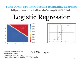
Logistic Regression Data: Inputs are continuous vectors of length M. Outputs are discrete. We are back to classification. Despite the name logistic regression. 32
Recall… Linear Models for Classification Key idea: Try to learn this hyperplane directly Looking ahead: Directly modeling the • We’ll see a number of hyperplane would use a commonly used Linear decision function: Classifiers • These include: h ( � ) = sign ( θ T � ) – Perceptron – Logistic Regression – Naïve Bayes (under for: certain conditions) – Support Vector y ∈ { − 1 , +1 } Machines
Recall… Background: Hyperplanes Hyperplane (Definition 1): Notation Trick : fold the H = { x : w T x = b } bias b and the weights w into a single vector θ by Hyperplane (Definition 2): prepending a constant to x and increasing dimensionality by one! w Half-spaces:
Using gradient ascent for linear classifiers Key idea behind today’s lecture: 1. Define a linear classifier (logistic regression) 2. Define an objective function (likelihood) 3. Optimize it with gradient descent to learn parameters 4. Predict the class with highest probability under the model 35
Using gradient ascent for linear classifiers This decision function isn’t Use a differentiable differentiable: function instead: 1 h ( � ) = sign ( θ T � ) p θ ( y = 1 | � ) = 1 + ��� ( − θ T � ) 1 sign(x) logistic( u ) ≡ 1 + e − u 36
Using gradient ascent for linear classifiers This decision function isn’t Use a differentiable differentiable: function instead: 1 h ( � ) = sign ( θ T � ) p θ ( y = 1 | � ) = 1 + ��� ( − θ T � ) 1 sign(x) logistic( u ) ≡ 1 + e − u 37
Logistic Regression Whiteboard – Logistic Regression Model – Learning for Logistic Regression • Partial derivative for Logistic Regression • Gradient for Logistic Regression 38
Recommend
More recommend
Explore More Topics
Stay informed with curated content and fresh updates.
