Regularization Jia-Bin Huang Virginia Tech Spring 2019 ECE-5424G - PowerPoint PPT Presentation

Regularization Jia-Bin Huang Virginia Tech Spring 2019 ECE-5424G / CS-5824

Administrative • Women in Data Science Blacksburg • Location: Holtzman Alumni Center • Welcome, 3:30 - 3:40, Assembly hall • Keynote Speaker: Milinda Lakkam, " Detecting automation on LinkedIn's platform ," 3:40 - 4:05, Assembly hall • Career Panel, 4:05 - 5:00, hall • Break , 5:00 - 5:20, Grand hallAssembly • Keynote Speaker: Sally Morton , " Bias ," 5:20 - 5:45, Assembly hall • Dinner with breakout discussion groups, 5:45 - 7:00, Museum • Introductory track tutorial: Jennifer Van Mullekom, " Data Visualization ", 7:00 - 8:15, Assembly hall • Advanced track tutorial: Cheryl Danner, " Focal-loss-based Deep Learning for Object Detection ," 7-8:15, 2nd floor board room

k-NN (Classification/Regression) • Model 𝑦 1 , 𝑧 1 , 𝑦 2 , 𝑧 2 , ⋯ , 𝑦 𝑛 , 𝑧 𝑛 • Cost function None • Learning Do nothing • Inference 𝑧 = ℎ 𝑦 test = 𝑧 (𝑙) , where 𝑙 = argmin 𝑗 𝐸(𝑦 test , 𝑦 (𝑗) ) ො

Linear regression (Regression) • Model ℎ 𝜄 𝑦 = 𝜄 0 + 𝜄 1 𝑦 1 + 𝜄 2 𝑦 2 + ⋯ + 𝜄 𝑜 𝑦 𝑜 = 𝜄 ⊤ 𝑦 • Cost function 𝑛 𝐾 𝜄 = 1 2 ℎ 𝜄 𝑦 𝑗 − 𝑧 𝑗 2𝑛 ෍ 𝑗=1 • Learning 𝑗 } 1 𝑛 ℎ 𝜄 𝑦 𝑗 − 𝑧 𝑗 𝑛 σ 𝑗=1 1) Gradient descent: Repeat { 𝜄 𝑘 ≔ 𝜄 𝑘 − 𝛽 𝑦 𝑘 2) Solving normal equation 𝜄 = (𝑌 ⊤ 𝑌) −1 𝑌 ⊤ 𝑧 • Inference 𝑧 = ℎ 𝜄 𝑦 test = 𝜄 ⊤ 𝑦 test ො

Naïve Bayes (Classification) • Model ℎ 𝜄 𝑦 = 𝑄(𝑍|𝑌 1 , 𝑌 2 , ⋯ , 𝑌 𝑜 ) ∝ 𝑄 𝑍 Π 𝑗 𝑄 𝑌 𝑗 𝑍) • Cost function Maximum likelihood estimation: 𝐾 𝜄 = − log 𝑄 Data 𝜄 Maximum a posteriori estimation : 𝐾 𝜄 = − log 𝑄 Data 𝜄 𝑄 𝜄 • Learning 𝜌 𝑙 = 𝑄(𝑍 = 𝑧 𝑙 ) (Discrete 𝑌 𝑗 ) 𝜄 𝑗𝑘𝑙 = 𝑄(𝑌 𝑗 = 𝑦 𝑗𝑘𝑙 |𝑍 = 𝑧 𝑙 ) 2 , 𝑄 𝑌 𝑗 𝑍 = 𝑧 𝑙 ) = 𝒪(𝑌 𝑗 |𝜈 𝑗𝑙 , 𝜏 𝑗𝑙 2 ) (Continuous 𝑌 𝑗 ) mean 𝜈 𝑗𝑙 , variance 𝜏 𝑗𝑙 • Inference test 𝑍 = 𝑧 𝑙 ) ෠ 𝑍 ← argmax 𝑄 𝑍 = 𝑧 𝑙 Π 𝑗 𝑄 𝑌 𝑗 𝑧 𝑙

Logistic regression (Classification) • Model 1 ℎ 𝜄 𝑦 = 𝑄 𝑍 = 1 𝑌 1 , 𝑌 2 , ⋯ , 𝑌 𝑜 = 1+𝑓 −𝜄⊤𝑦 • Cost function 𝑛 𝐾 𝜄 = 1 Cost(ℎ 𝜄 𝑦 , 𝑧) = ൝−log ℎ 𝜄 𝑦 if 𝑧 = 1 Cost(ℎ 𝜄 (𝑦 𝑗 ), 𝑧 (𝑗) )) 𝑛 ෍ −log 1 − ℎ 𝜄 𝑦 if 𝑧 = 0 𝑗=1 • Learning 𝑗 } 1 𝑛 ℎ 𝜄 𝑦 𝑗 − 𝑧 𝑗 𝑛 σ 𝑗=1 Gradient descent: Repeat { 𝜄 𝑘 ≔ 𝜄 𝑘 − 𝛽 𝑦 𝑘 • Inference 1 𝑍 = ℎ 𝜄 𝑦 test = ෠ 1 + 𝑓 −𝜄 ⊤ 𝑦 test

Logistic Regression 1 • Hypothesis representation ℎ 𝜄 𝑦 = 1 + 𝑓 −𝜄 ⊤ 𝑦 Cost(ℎ 𝜄 𝑦 , 𝑧) = ൝ −log ℎ 𝜄 𝑦 if 𝑧 = 1 • Cost function −log 1 − ℎ 𝜄 𝑦 if 𝑧 = 0 • Logistic regression with gradient descent 𝑛 𝑘 − 𝛽 1 − 𝑧 (𝑗) 𝑦 𝑘 (𝑗) ℎ 𝜄 𝑦 𝑗 𝜄 𝑘 ≔ 𝜄 𝑛 ෍ • Regularization 𝑗=1 • Multi-class classification

How about MAP? • Maximum conditional likelihood estimate (MCLE) 𝑛 𝑄 𝜄 𝑧 (𝑗) |𝑦 𝑗 ς 𝑗=1 𝜄 MCLE = argmax 𝜄 • Maximum conditional a posterior estimate (MCAP) 𝑛 𝑄 𝜄 𝑧 (𝑗) |𝑦 𝑗 ς 𝑗=1 𝜄 MCAP = argmax 𝑄(𝜄) 𝜄

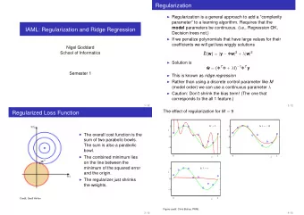
Prior 𝑄(𝜄) • Common choice of 𝑄(𝜄) : • Normal distribution, zero mean, identity covariance • “Pushes” parameters towards zeros • Corresponds to Regularization • Helps avoid very large weights and overfitting Slide credit: Tom Mitchell

MLE vs. MAP • Maximum conditional likelihood estimate (MCLE) 𝑛 𝑘 − 𝛽 1 − 𝑧 (𝑗) 𝑦 𝑘 (𝑗) ℎ 𝜄 𝑦 𝑗 𝜄 𝑘 ≔ 𝜄 𝑛 ෍ 𝑗=1 • Maximum conditional a posterior estimate (MCAP) 𝑛 𝑘 − 𝛽 1 − 𝑧 (𝑗) 𝑦 𝑘 (𝑗) ℎ 𝜄 𝑦 𝑗 𝜄 𝑘 ≔ 𝜄 𝑘 − 𝛽𝜇𝜄 𝑛 ෍ 𝑗=1

Logistic Regression • Hypothesis representation • Cost function • Logistic regression with gradient descent • Regularization • Multi-class classification

Multi-class classification • Email foldering/taggning: Work, Friends, Family, Hobby • Medical diagrams: Not ill, Cold, Flu • Weather: Sunny, Cloudy, Rain, Snow Slide credit: Andrew Ng

Binary classification Multiclass classification 𝑦 2 𝑦 2 𝑦 1 𝑦 1

One-vs-all (one-vs-rest) 𝑦 2 1 𝑦 ℎ 𝜄 𝑦 1 𝑦 2 𝑦 2 2 𝑦 ℎ 𝜄 𝑦 1 𝑦 1 Class 1: Class 2: 𝑦 2 3 𝑦 ℎ 𝜄 Class 3: 𝑗 𝑦 = 𝑄 𝑧 = 𝑗 𝑦; 𝜄 ℎ 𝜄 (𝑗 = 1, 2, 3) 𝑦 1 Slide credit: Andrew Ng

One-vs-all 𝑗 𝑦 for • Train a logistic regression classifier ℎ 𝜄 each class 𝑗 to predict the probability that 𝑧 = 𝑗 • Given a new input 𝑦 , pick the class 𝑗 that maximizes 𝑗 𝑦 max ℎ 𝜄 i Slide credit: Andrew Ng

Generative Approach Discriminative Approach Ex: Naïve Bayes Ex: Logistic regression Estimate 𝑄(𝑍) and 𝑄(𝑌|𝑍) Estimate 𝑄(𝑍|𝑌) directly (Or a discriminant function: e.g., SVM) Prediction Prediction 𝑧 = argmax 𝑧 𝑄 𝑍 = 𝑧 𝑄(𝑌 = 𝑦|𝑍 = 𝑧) 𝑧 = 𝑄(𝑍 = 𝑧|𝑌 = 𝑦) ො ො

Further readings • Tom M. Mitchell Generative and discriminative classifiers: Naïve Bayes and Logistic Regression http://www.cs.cmu.edu/~tom/mlbook/NBayesLogReg.pdf • Andrew Ng, Michael Jordan On discriminative vs. generative classifiers: A comparison of logistic regression and naive bayes http://papers.nips.cc/paper/2020-on-discriminative-vs-generative- classifiers-a-comparison-of-logistic-regression-and-naive-bayes.pdf

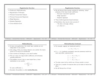
Regularization • Overfitting • Cost function • Regularized linear regression • Regularized logistic regression

Regularization • Overfitting • Cost function • Regularized linear regression • Regularized logistic regression

Example: Linear regression Price ($) Price ($) Price ($) in 1000’s in 1000’s in 1000’s Size in feet^2 Size in feet^2 Size in feet^2 ℎ 𝜄 𝑦 = 𝜄 0 + 𝜄 1 𝑦 + 𝜄 2 𝑦 2 + ℎ 𝜄 𝑦 = 𝜄 0 + 𝜄 1 𝑦 + 𝜄 2 𝑦 2 ℎ 𝜄 𝑦 = 𝜄 0 + 𝜄 1 𝑦 𝜄 3 𝑦 3 + 𝜄 4 𝑦 4 + ⋯ Underfitting Just right Overfitting Slide credit: Andrew Ng

Overfitting • If we have too many features (i.e. complex model), the learned hypothesis may fit the training set very well 𝑛 𝐾 𝜄 = 1 2 ≈ 0 ℎ 𝜄 𝑦 𝑗 − 𝑧 𝑗 2𝑛 ෍ 𝑗=1 but fail to generalize to new examples (predict prices on new examples). Slide credit: Andrew Ng

Example: Linear regression Price ($) Price ($) Price ($) in 1000’s in 1000’s in 1000’s Size in feet^2 Size in feet^2 Size in feet^2 ℎ 𝜄 𝑦 = 𝜄 0 + 𝜄 1 𝑦 + 𝜄 2 𝑦 2 + ℎ 𝜄 𝑦 = 𝜄 0 + 𝜄 1 𝑦 + 𝜄 2 𝑦 2 ℎ 𝜄 𝑦 = 𝜄 0 + 𝜄 1 𝑦 𝜄 3 𝑦 3 + 𝜄 4 𝑦 4 + ⋯ Underfitting Just right Overfitting High bias High variance Slide credit: Andrew Ng

Bias-Variance Tradeoff • Bias : difference between what you expect to learn and truth • Measures how well you expect to represent true solution • Decreases with more complex model • Variance : difference between what you expect to learn and what you learn from a particular dataset • Measures how sensitive learner is to specific dataset • Increases with more complex model

Low variance High variance Low bias High bias

Bias – variance decomposition • Training set { 𝑦 1 , 𝑧 1 , 𝑦 2 , 𝑧 2 , ⋯ , 𝑦 𝑜 , 𝑧 𝑜 } • 𝑧 = 𝑔 𝑦 + 𝜁 2 • We want መ 𝑧 − መ 𝑔 𝑦 that minimizes 𝐹 𝑔 𝑦 2 2 + Var መ 𝑧 − መ = Bias መ + 𝜏 2 𝐹 𝑔 𝑦 𝑔 𝑦 𝑔 𝑦 Bias መ = 𝐹 መ 𝑔 𝑦 𝑔 𝑦 − 𝑔(𝑦) 2 𝑔 𝑦 2 − 𝐹 መ Var መ = 𝐹 መ 𝑔 𝑦 𝑔 𝑦 https://en.wikipedia.org/wiki/Bias%E2%80%93variance_tradeoff

Overfitting Age Age Age Tumor Size Tumor Size Tumor Size ℎ 𝜄 𝑦 = 𝑕(𝜄 0 + 𝜄 1 𝑦 + 𝜄 2 𝑦 2 ) ℎ 𝜄 𝑦 = 𝑕(𝜄 0 + 𝜄 1 𝑦 + 𝜄 2 𝑦 2 + ℎ 𝜄 𝑦 = 𝑕(𝜄 0 + 𝜄 1 𝑦 + 𝜄 2 𝑦 2 + 2 + 𝜄 4 𝑦 2 2 + 𝜄 5 𝑦 1 𝑦 2 ) 2 + 𝜄 4 𝑦 2 2 + 𝜄 5 𝑦 1 𝑦 2 + 𝜄 3 𝑦 1 𝜄 3 𝑦 1 3 + ⋯ ) 3 𝑦 2 + 𝜄 7 𝑦 1 𝑦 2 𝜄 6 𝑦 1 Underfitting Overfitting Slide credit: Andrew Ng

Addressing overfitting Price ($) • 𝑦 1 = size of house in 1000’s • 𝑦 2 = no. of bedrooms • 𝑦 3 = no. of floors • 𝑦 4 = age of house • 𝑦 5 = average income in neighborhood Size in feet^2 • 𝑦 6 = kitchen size • ⋮ • 𝑦 100 Slide credit: Andrew Ng

Addressing overfitting • 1. Reduce number of features. • Manually select which features to keep. • Model selection algorithm (later in course). • 2. Regularization. • Keep all the features, but reduce magnitude/values of parameters 𝜄 𝑘 . • Works well when we have a lot of features, each of which contributes a bit to predicting 𝑧 . Slide credit: Andrew Ng

Overfitting Thriller • https://www.youtube.com/watch?v=DQWI1kvmwRg

Regularization • Overfitting • Cost function • Regularized linear regression • Regularized logistic regression