[PPT] - CS7015 (Deep Learning) : Lecture 8 Regularization: Bias Variance PowerPoint Presentation

SLIDE 1

1/1

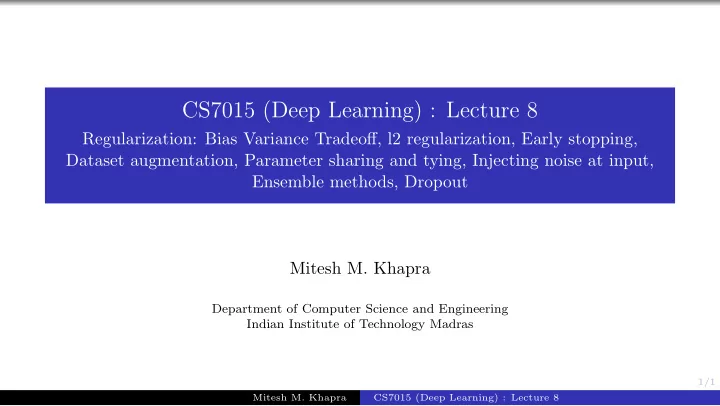
CS7015 (Deep Learning) : Lecture 8

Regularization: Bias Variance Tradeoff, l2 regularization, Early stopping, Dataset augmentation, Parameter sharing and tying, Injecting noise at input, Ensemble methods, Dropout Mitesh M. Khapra

Department of Computer Science and Engineering Indian Institute of Technology Madras

Mitesh M. Khapra CS7015 (Deep Learning) : Lecture 8

SLIDE 2

2/1

Acknowledgements Chapter 7, Deep Learning book Ali Ghodsi’s Video Lectures on Regularizationa Dropout: A Simple Way to Prevent Neural Networks from Overfittingb

aLecture 2.1 and Lecture 2.2 bDropout Mitesh M. Khapra CS7015 (Deep Learning) : Lecture 8

SLIDE 3

3/1

Module 8.1 : Bias and Variance

Mitesh M. Khapra CS7015 (Deep Learning) : Lecture 8

SLIDE 4

4/1

We will begin with a quick overview of bias, variance and the trade-off between them.

Mitesh M. Khapra CS7015 (Deep Learning) : Lecture 8

SLIDE 5

5/1

Simple Complex The points were drawn from a si- nusoidal function (the true f(x)) Let us consider the problem of fitting a curve through a given set of points We consider two models :

Simple (degree:1)

y = ˆ f(x) = w1x + w0

Complex (degree:25)

y = ˆ f(x) =

25

i=1

wixi + w0 Note that in both cases we are making an as- sumption about how y is related to x. We have no idea about the true relation f(x) The training data consists of 100 points

Mitesh M. Khapra CS7015 (Deep Learning) : Lecture 8

SLIDE 6

6/1

Simple Complex The points were drawn from a sinusoidal function (the true f(x)) We sample 25 points from the training data and train a simple and a complex model We repeat the process ‘k’ times to train multiple models (each model sees a different sample of the training data) We make a few observations from these plots

Mitesh M. Khapra CS7015 (Deep Learning) : Lecture 8

SLIDE 7

7/1 Mitesh M. Khapra CS7015 (Deep Learning) : Lecture 8

SLIDE 8

8/1

Simple models trained on different samples of the data do not differ much from each other However they are very far from the true sinus-

idal curve (under fitting)

On the other hand, complex models trained on different samples of the data are very different from each other (high variance)

Mitesh M. Khapra CS7015 (Deep Learning) : Lecture 8

SLIDE 9

9/1

Green Line: Average value of ˆ f(x) for the simple model Blue Curve: Average value of ˆ f(x) for the complex model Red Curve: True model (f(x))

Let f(x) be the true model (sinusoidal in this case) and ˆ f(x) be our estimate of the model (simple or complex, in this case) then, Bias ( ˆ f(x)) = E[ ˆ f(x)] − f(x) E[ ˆ f(x)] is the average (or expected) value of the model We can see that for the simple model the av- erage value (green line) is very far from the true value f(x) (sinusoidal function) Mathematically, this means that the simple model has a high bias On the other hand, the complex model has a low bias

Mitesh M. Khapra CS7015 (Deep Learning) : Lecture 8

SLIDE 10

10/1

We now define, Variance ( ˆ f(x)) = E[( ˆ f(x) − E[ ˆ f(x)])2] (Standard definition from statistics) Roughly speaking it tells us how much the dif- ferent ˆ f(x)’s (trained on different samples of the data) differ from each other It is clear that the simple model has a low vari- ance whereas the complex model has a high variance

Mitesh M. Khapra CS7015 (Deep Learning) : Lecture 8

SLIDE 11

11/1

In summary (informally) Simple model: high bias, low variance Complex model: low bias, high variance There is always a trade-off between the bias and variance Both bias and variance contribute to the mean square error. Let us see how

Mitesh M. Khapra CS7015 (Deep Learning) : Lecture 8

SLIDE 12

12/1

Module 8.2 : Train error vs Test error

Mitesh M. Khapra CS7015 (Deep Learning) : Lecture 8

SLIDE 13

13/1

We can show that E[(y − ˆ f(x))2] = Bias2 + V ariance + σ2 (irreducible error) See proof here Consider a new point (x, y) which was not seen during training If we use the model ˆ f(x) to predict the value of y then the mean square error is given by E[(y − ˆ f(x))2] (average square error in predicting y for many such unseen points)

Mitesh M. Khapra CS7015 (Deep Learning) : Lecture 8

SLIDE 14

14/1

model complexity error High bias High variance Sweet spot-

perfect tradeoff
ideal model

complexity E[(y − ˆ f(x))2] = Bias2 + V ariance + σ2 (irreducible error) The parameters of ˆ f(x) (all wi’s) are trained using a training set {(xi, yi)}n

i=1

However, at test time we are interested in eval- uating the model on a validation (unseen) set which was not used for training This gives rise to the following two entities of interest: trainerr (say, mean square error) testerr (say, mean square error) Typically these errors exhibit the trend shown in the adjacent figure

Mitesh M. Khapra CS7015 (Deep Learning) : Lecture 8

SLIDE 15

15/1

Intuitions developed so far Let there be n training points and m test (validation) points trainerr = 1 n

n

i=1

(yi − ˆ f(xi))2 testerr = 1 m

n+m

i=n+1

(yi − ˆ f(xi))2 As the model complexity increases trainerr becomes overly optimistic and gives us a wrong picture of how close ˆ f is to f The validation error gives the real picture of how close ˆ f is to f We will concretize this intuition mathematically now and eventually show how to account for the optimism in the training error

Mitesh M. Khapra CS7015 (Deep Learning) : Lecture 8

SLIDE 16

16/1

Let D={xi, yi}m+n

i=1 ,

then for any point (x, y) we have, yi = f(xi) + εi which means that yi is related to xi by some true function f but there is also some noise ε in the relation For simplicity, we assume ε ∼ N(0, σ2) and of course we do not know f Further we use ˆ f to approximate f and estimate the parameters using T ⊂ D such that yi = ˆ f(xi) We are interested in knowing E[( ˆ f(xi) − f(xi))2] but we cannot estimate this directly because we do not know f We will see how to estimate this em- pirically using the observation yi & prediction ˆ yi

Mitesh M. Khapra CS7015 (Deep Learning) : Lecture 8

SLIDE 17

17/1

E[( ˆ yi − yi)2] = E[( ˆ f(xi) − f(xi) − εi)2] (yi = f(xi) + εi) = E[( ˆ f(xi) − f(xi))2 − 2εi( ˆ f(xi) − f(xi)) + ε2

i ]

= E[( ˆ f(xi) − f(xi))2] − 2E[εi( ˆ f(xi) − f(xi))] + E[ε2

i ]

∴ E[( ˆ f(xi) − f(xi))2] = E[( ˆ yi − yi)2] − E[ε2

i ] + 2E[ εi( ˆ

f(xi) − f(xi)) ]

Mitesh M. Khapra CS7015 (Deep Learning) : Lecture 8

SLIDE 18

18/1

We will take a small detour to understand how to empirically estimate an Expectation and then return to our derivation

Mitesh M. Khapra CS7015 (Deep Learning) : Lecture 8

SLIDE 19

19/1

Suppose we have observed the goals scored(z) in k matches as z1 = 2, z2 = 1, z3 = 0, ... zk = 2 Now we can empirically estimate E[z] i.e. the expected number of goals scored as E[z] = 1 k

k

i=1

zi Analogy with our derivation: We have a certain number of observations yi & predictions ˆ yi using which we can estimate E[( ˆ yi − yi)2] = 1 m

m

i=1

( ˆ yi − yi)2

Mitesh M. Khapra CS7015 (Deep Learning) : Lecture 8

SLIDE 20

20/1

... returning back to our derivation

Mitesh M. Khapra CS7015 (Deep Learning) : Lecture 8

SLIDE 21

21/1

E[( ˆ f(xi) − f(xi))2] = E[( ˆ yi − yi)2] − E[ε2

i ] + 2E[ εi( ˆ

f(xi) − f(xi)) ] We can empirically evaluate R.H.S using training observations or test observa- tions Case 1: Using test observations

E[( ˆ f(xi) − f(xi))2]

true error

= 1 m

n+m

i=n+1

( ˆ yi − yi)2

empirical estimation of error

− 1 m

n+m

i=n+1

ε2

i

small constant

+ 2 E[ εi( ˆ f(xi) − f(xi)) ]

= covariance (εi, ˆ

f(xi)−f(xi))

∵ covariance(X, Y ) = E[(X − µX)(Y − µY )] = E[(X)(Y − µY )](if µX = E[X] = 0) = E[XY ] − E[XµY ] = E[XY ] − µY E[X] = E[XY ]

Mitesh M. Khapra CS7015 (Deep Learning) : Lecture 8

SLIDE 22

22/1

E[( ˆ f(xi) − f(xi))2]

true error

= 1 m

n+m

i=n+1

( ˆ yi − yi)2

empirical estimation of error

− 1 m

n+m

i=n+1

ε2

i

small constant

+ 2 E[ εi( ˆ f(xi) − f(xi)) ]

= covariance (εi, ˆ

f(xi)−f(xi))

None of the test observations participated in the estimation of ˆ f(x)[the para- meters of ˆ f(x) were estimated only using training data] ∴ ε ⊥ ( ˆ f(xi) − f(xi)) ∴ E[εi · ( ˆ f(xi) − f(xi))] = E[εi] · E[ ˆ f(xi) − f(xi))] = 0 · E[ ˆ f(xi) − f(xi))] = 0 ∴ true error = empirical test error + small constant Hence, we should always use a validation set(independent of the training set) to estimate the error

Mitesh M. Khapra CS7015 (Deep Learning) : Lecture 8

SLIDE 23

23/1

Case 2: Using training observations E[( ˆ f(xi) − f(xi))2]

true error

= 1 n

n

i=1

( ˆ yi − yi)2

empirical estimation of error

− 1 n

n

i=1

ε2

i

small constant

+ 2 E[ εi( ˆ f(xi) − f(xi)) ]

= covariance (εi, ˆ

f(xi)−f(xi))

Now, ε ⊥ ˆ f(x) because ε was used for estimating the parameters of ˆ f(x) ∴ E[εi · ( ˆ f(xi) − f(xi))] = E[εi] · E[ ˆ f(xi) − f(xi))] = 0 Hence, the empirical train error is smaller than the true error and does not give a true picture of the error But how is this related to model complexity? Let us see

Mitesh M. Khapra CS7015 (Deep Learning) : Lecture 8

SLIDE 24

24/1

Module 8.3 : True error and Model complexity

Mitesh M. Khapra CS7015 (Deep Learning) : Lecture 8

SLIDE 25

25/1

Using Stein’s Lemma (and some trickery) we can show that 1 n

n

i=1

εi( ˆ f(xi) − f(xi)) = σ2 n

n

i=1

∂ ˆ f(xi) ∂yi When will ∂ ˆ

f(xi) ∂yi

be high? When a small change in the observation causes a large change in the estimation( ˆ f) Can you link this to model complexity? Yes, indeed a complex model will be more sensitive to changes in observations whereas a simple model will be less sensitive to changes in observations Hence, we can say that true error = empirical train error + small constant + Ω(model complexity)

Mitesh M. Khapra CS7015 (Deep Learning) : Lecture 8

SLIDE 26

26/1 Mitesh M. Khapra CS7015 (Deep Learning) : Lecture 8

SLIDE 27

27/1

Let us verify that indeed a complex model is more sens- itive to minor changes in the data We have fitted a simple and complex model for some given data We now change one of these data points The simple model does not change much as compared to the complex model

Mitesh M. Khapra CS7015 (Deep Learning) : Lecture 8

SLIDE 28

28/1

Hence while training, instead of minimizing the training error Ltrain(θ) we should minimize min

w.r.t θ Ltrain(θ) + Ω(θ) = L (θ)

Where Ω(θ) would be high for complex models and small for simple models Ω(θ) acts as an approximate for σ2

n

i=1 ∂ ˆ f(xi) ∂yi

This is the basis for all regularization methods We can show that l1 regularization, l2 regularization, early stopping and inject- ing noise in input are all instances of this form of regularization.

Mitesh M. Khapra CS7015 (Deep Learning) : Lecture 8

SLIDE 29

29/1

model complexity error High bias High variance Sweet spot Ω(θ) should ensure that model has reas-

nable complexity

σ2 n

n

i=1 ∂ ˆ f(xi) ∂yi

Mitesh M. Khapra CS7015 (Deep Learning) : Lecture 8

SLIDE 30

30/1

Why do we care about this bias variance tradeoff and model complexity? Deep Neural networks are highly complex models. Many parameters, many non-linearities. It is easy for them to overfit and drive training error to 0. Hence we need some form of regularization.

Mitesh M. Khapra CS7015 (Deep Learning) : Lecture 8

SLIDE 31

31/1

Different forms of regularization l2 regularization Dataset augmentation Parameter Sharing and tying Adding Noise to the inputs Adding Noise to the outputs Early stopping Ensemble methods Dropout

Mitesh M. Khapra CS7015 (Deep Learning) : Lecture 8

SLIDE 32

32/1

Module 8.4 : l2 regularization

Mitesh M. Khapra CS7015 (Deep Learning) : Lecture 8

SLIDE 33

33/1

Different forms of regularization l2 regularization Dataset augmentation Parameter Sharing and tying Adding Noise to the inputs Adding Noise to the outputs Early stopping Ensemble methods Dropout

Mitesh M. Khapra CS7015 (Deep Learning) : Lecture 8

SLIDE 34

34/1

For l2 regularization we have,

L (w) = L (w) + α

2 w2 For SGD (or its variants), we are interested in ∇ L (w) = ∇L (w) + αw Update rule: wt+1 = wt − η∇L (wt) − ηαwt Requires a very small modification to the code Let us see the geometric interpretation of this

Mitesh M. Khapra CS7015 (Deep Learning) : Lecture 8

SLIDE 35

35/1

Assume w∗ is the optimal solution for L (w) [not L (w)] i.e. the solution in the absence of regularization (w∗ optimal → ∇L (w∗) = 0) Consider u = w − w∗. Using Taylor series approximation (upto 2nd order) L (w∗ + u) = L (w∗) + uT ∇L (w∗) + 1 2uT Hu L (w) = L (w∗) + (w − w∗)T ∇L (w∗) + 1 2(w − w∗)T H(w − w∗) = L (w∗) + 1 2(w − w∗)T H(w − w∗) (∵ ∇L(w∗) = 0 ) ∇L (w) = ∇L (w∗) + H(w − w∗) = H(w − w∗) Now, ∇ L (w) = ∇L (w) + αw = H(w − w∗) + αw

Mitesh M. Khapra CS7015 (Deep Learning) : Lecture 8

SLIDE 36

36/1

Let w be the optimal solution for L(w) [i.e regularized loss] ∵ ∇ L( w) = 0 H( w − w∗) + α w = 0 ∴(H + αI) w = Hw∗ ∴ w = (H + αI)−1Hw∗ Notice that if α → 0 then w → w∗ [no regularization] But we are interested in the case when α = 0 Let us analyse the case when α = 0

Mitesh M. Khapra CS7015 (Deep Learning) : Lecture 8

SLIDE 37

37/1

If H is symmetric Positive Semi Definite H = QΛQT [Q is orthogonal, QQT = QT Q = I]

w = (H + αI)−1Hw∗

= (QΛQT + αI)−1QΛQT w∗ = (QΛQT + αQIQT )−1QΛQT w∗ = [Q(Λ + αI)QT ]−1QΛQT w∗ = QT −1(Λ + αI)−1Q−1QΛQT w∗ = Q(Λ + αI)−1ΛQT w∗ (∵ QT −1 = Q)

w = QDQT w∗

where D = (Λ + αI)−1Λ, is a diagonal matrix which we will see in more detail soon

Mitesh M. Khapra CS7015 (Deep Learning) : Lecture 8

SLIDE 38

38/1

w = Q(Λ + αI)−1ΛQT w∗

= QDQT w∗ (Λ + αI)−1 =     

1 λ1+α 1 λ2+α

...

1 λn+α

     D = (Λ + αI)−1Λ (Λ + αI)−1Λ =     

λ1 λ1+α λ2 λ2+α

...

λn λn+α

     So what is happening here? w∗ first gets rotated by QT to give QT w∗ However if α = 0 then Q rotates QT w∗ back to give w∗ If α = 0 then let us see what D looks like So what is happening now?

Mitesh M. Khapra CS7015 (Deep Learning) : Lecture 8

SLIDE 39

39/1

w = Q(Λ + αI)−1ΛQT w∗

= QDQT w∗ (Λ + αI)−1 =     

1 λ1+α 1 λ2+α

...

1 λn+α

     D = (Λ + αI)−1Λ (Λ + αI)−1Λ =     

λ1 λ1+α λ2 λ2+α

...

λn λn+α

     Each element i of QT w∗ gets scaled by

λi λi+α before it is rotated back by

Q if λi >> α then

λi λi+α = 1

if λi << α then

λi λi+α = 0

Thus only significant directions (larger eigen values) will be retained. Effective parameters =

n

i=1

λi λi + α < n

Mitesh M. Khapra CS7015 (Deep Learning) : Lecture 8

SLIDE 40

40/1

The weight vector(w∗) is getting rotated to ( ˜ w) All of its elements are shrinking but some are shrinking more than the others This ensures that only important features are given high weights

Mitesh M. Khapra CS7015 (Deep Learning) : Lecture 8

SLIDE 41

41/1

Module 8.5 : Dataset augmentation

Mitesh M. Khapra CS7015 (Deep Learning) : Lecture 8

SLIDE 42

42/1

Different forms of regularization l2 regularization Dataset augmentation Parameter Sharing and tying Adding Noise to the inputs Adding Noise to the outputs Early stopping Ensemble methods Dropout

Mitesh M. Khapra CS7015 (Deep Learning) : Lecture 8

SLIDE 43

43/1

label = 2 [given training data] We exploit the fact that certain transformations to the image do not change the label of the image. label = 2 rotated by 20◦ rotated by 65◦ shifted vertically shifted horizontally blurred changed some pixels [augmented data = created using some knowledge of the task]

Mitesh M. Khapra CS7015 (Deep Learning) : Lecture 8

SLIDE 44

44/1

Typically, More data = better learning Works well for image classification / object recognition tasks Also shown to work well for speech For some tasks it may not be clear how to generate such data

Mitesh M. Khapra CS7015 (Deep Learning) : Lecture 8

SLIDE 45

45/1

Module 8.6 : Parameter Sharing and tying

Mitesh M. Khapra CS7015 (Deep Learning) : Lecture 8

SLIDE 46

46/1

Other forms of regularization l2 regularization Dataset augmentation Parameter Sharing and tying Adding Noise to the inputs Adding Noise to the outputs Early stopping Ensemble methods Dropout

Mitesh M. Khapra CS7015 (Deep Learning) : Lecture 8

SLIDE 47

47/1

Parameter Sharing Used in CNNs Same filter applied at different positions of the image Or same weight matrix acts on different input neurons x h(x) ˆ x Parameter Tying Typically used in autoencoders The encoder and decoder weights are tied.

Mitesh M. Khapra CS7015 (Deep Learning) : Lecture 8

SLIDE 48

48/1

Module 8.7 : Adding Noise to the inputs

Mitesh M. Khapra CS7015 (Deep Learning) : Lecture 8

SLIDE 49

49/1

Other forms of regularization l2 regularization Dataset augmentation Parameter Sharing and tying Adding Noise to the inputs Adding Noise to the outputs Early stopping Ensemble methods Dropout

Mitesh M. Khapra CS7015 (Deep Learning) : Lecture 8

SLIDE 50

50/1

x ˜ x h(x) ˆ x P(˜ x|x) ←noise process We saw this in Autoencoder We can show that for a simple input

utput neural network, adding Gaus-

sian noise to the input is equivalent to weight decay (L2 regularisation) Can be viewed as data augmentation

Mitesh M. Khapra CS7015 (Deep Learning) : Lecture 8

SLIDE 51

51/1 x1 + ε1 x2 + ε2

. . .

xk + εk

. . .

xn + εn

ε ∼ N(0, σ2)

xi = xi + εi
y =

n

i=1

wixi

y =

n

i=1

wi xi =

n

i=1

wixi +

n

i=1

wiεi = y +

n

i=1

wiεi We are interested in E[( y − y)2] E

(

y − y)2 = E

y +

n

i=1

wiεi − y 2

= E

 

y − y
+
n
i=1

wiεi 2  = E

(

y − y)2 + E

2(

y − y)

n

i=1

wiεi

+ E
n
i=1

wiεi 2

= E
(

y − y)2 + 0 + E n

i=1

w2

i ε2 i

(∵ εi is independent of εj and εi is independent of (

y-y) ) = (E

(

y − y)2 + σ2

n

i=1

w2

i

(same as L2 norm penalty)

Mitesh M. Khapra CS7015 (Deep Learning) : Lecture 8

SLIDE 52

52/1

Module 8.8 : Adding Noise to the outputs

Mitesh M. Khapra CS7015 (Deep Learning) : Lecture 8

SLIDE 53

53/1

Other forms of regularization l2 regularization Dataset augmentation Parameter Sharing and tying Adding Noise to the inputs Adding Noise to the outputs Early stopping Ensemble methods Dropout

Mitesh M. Khapra CS7015 (Deep Learning) : Lecture 8

SLIDE 54

54/1

Hard targets 1 minimize :

9

i=0

pi log qi true distribution : p = {0, 0, 1, 0, 0, 0, 0, 0, 0, 0} estimated distribution : q Intuition Do not trust the true labels, they may be noisy Instead, use soft targets

Mitesh M. Khapra CS7015 (Deep Learning) : Lecture 8

SLIDE 55

55/1

Soft targets

ε 9 ε 9

1 − ε

ε 9 ε 9 ε 9 ε 9 ε 9 ε 9 ε 9

ε = small positive constant minimize :

9

i=0

pi log qi true distribution + noise : p = ε 9, ε 9, 1 − ε, ε 9, . . .

estimated distribution : q

Mitesh M. Khapra CS7015 (Deep Learning) : Lecture 8

SLIDE 56

56/1

Module 8.9 : Early stopping

Mitesh M. Khapra CS7015 (Deep Learning) : Lecture 8

SLIDE 57

57/1

Other forms of regularization l2 regularization Dataset augmentation Parameter Sharing and tying Adding Noise to the inputs Adding Noise to the outputs Early stopping Ensemble methods Dropout

Mitesh M. Khapra CS7015 (Deep Learning) : Lecture 8

SLIDE 58

58/1 Steps Error T raining error V alidation error k − p k stop return this model

Track the validation error Have a patience parameter p If you are at step k and there was no improvement in validation error in the previous p steps then stop train- ing and return the model stored at step k − p Basically, stop the training early be- fore it drives the training error to 0 and blows up the validation error

Mitesh M. Khapra CS7015 (Deep Learning) : Lecture 8

SLIDE 59

59/1 Steps Error T raining error V alidation error k − p k stop return this model

Very effective and the mostly widely used form of regularization Can be used even with other regular- izers (such as l2) How does it act as a regularizer ? We will first see an intuitive explan- ation and then a mathematical ana- lysis

Mitesh M. Khapra CS7015 (Deep Learning) : Lecture 8

SLIDE 60

60/1 Steps Error T raining error V alidation error k − p k stop return this model

Recall that the update rule in SGD is wt+1 = wt − η∇wt = w0 − η

t

i=1

∇wi Let τ be the maximum value of ∇wi then |wt+1 − w0| ≤ ηt|τ| Thus, t controls how far wt can go from the initial w0 In other words it controls the space

f exploration

Mitesh M. Khapra CS7015 (Deep Learning) : Lecture 8

SLIDE 61

61/1

We will now see a mathematical analysis of this

Mitesh M. Khapra CS7015 (Deep Learning) : Lecture 8

SLIDE 62

62/1

Recall that the Taylor series approximation for L (w) is L (w) = L (w∗) + (w − w∗)T ∇L (w∗) + 1 2(w − w∗)T H(w − w∗) = L (w∗) + 1 2(w − w∗)T H(w − w∗) [ w∗ is optimal so ∇L (w∗) is 0 ] ∇(L (w)) = H(w − w∗) Now the SGD update rule is: wt = wt−1 − η∇L (wt−1) = wt−1 − ηH(wt−1 − w∗) = (I − ηH)wt−1 + ηHw∗

Mitesh M. Khapra CS7015 (Deep Learning) : Lecture 8

SLIDE 63

63/1

wt = (I − ηH)wt−1 + ηHw∗ Using EVD of H as H = QΛQT , we get: wt = (I − ηQΛQT )wt−1 + ηQΛQT w∗ If we start with w0 = 0 then we can show that (See Appendix) wt = Q[I − (I − εΛ)t]QT w∗ Compare this with the expression we had for optimum ˜ W with L2 regularization ˜ w = Q[I − (Λ + αI)−1α]QT w∗ We observe that wt = ˜ w, if we choose ε,t and α such that (I − εΛ)t = (Λ + αI)−1α

Mitesh M. Khapra CS7015 (Deep Learning) : Lecture 8

SLIDE 64

64/1

Things to be remember Early stopping only allows t updates to the parameters. If a parameter w corresponds to a dimension which is important for the loss L (θ) then ∂L (θ)

∂w

will be large However if a parameter is not important ( ∂L (θ)

∂w

is small) then its updates will be small and the parameter will not be able to grow large in ‘t′ steps Early stopping will thus effectively shrink the parameters corresponding to less important directions (same as weight decay).

Mitesh M. Khapra CS7015 (Deep Learning) : Lecture 8

SLIDE 65

65/1

Module 8.10 : Ensemble methods

Mitesh M. Khapra CS7015 (Deep Learning) : Lecture 8

SLIDE 66

66/1

Other forms of regularization l2 regularization Dataset augmentation Parameter Sharing and tying Adding Noise to the inputs Adding Noise to the outputs Early stopping Ensemble methods Dropout

Mitesh M. Khapra CS7015 (Deep Learning) : Lecture 8

SLIDE 67

67/1

y ylr Logistic Regression ysvm SV M ynb x1 x2 x3 x4 y Naive Bayes yfinal

Combine the output of different models to re- duce generalization error The models can correspond to different clas- sifiers It could be different instances of the same clas- sifier trained with:

different hyperparameters different features different samples of the training data

Mitesh M. Khapra CS7015 (Deep Learning) : Lecture 8

SLIDE 68

68/1

y ylr1 y ylr2 y ylr3 Logistic Logistic Logistic Regression Regression Regression yfinal

Each model trained with a different sample of the data (sampling with replacement) Bagging: form an ensemble using dif- ferent instances of the same classifier From a given dataset, construct mul- tiple training sets by sampling with replacement (T1, T2, ..., Tk) Train ith instance of the classifier us- ing training set Ti

Mitesh M. Khapra CS7015 (Deep Learning) : Lecture 8

SLIDE 69

69/1

The error made by the average prediction of all the models is

1 k

i εi

The expected squared error is :

mse =E[(1 k

i

εi)2] = 1 k2 E[

i
i=j

εiεj +

i
i=j

εiεj] = 1 k2 E[

i

ε2

i +

i
i=j

εiεj] = 1 k2 (

i

E[ε2

i ] +

i
i=j

E[εiεj]) = 1 k2 (kV + k(k − 1)C) =1 kV + k − 1 k C

When would bagging work? Consider a set of k LR mod- els Suppose that each model makes an error εi on a test example Let εi be drawn from a zero mean multivariate nor- mal distribution V ariance = E[ε2

i ] = V

Covariance = E[εiεj] = C

Mitesh M. Khapra CS7015 (Deep Learning) : Lecture 8

SLIDE 70

70/1

mse = 1 kV + k − 1 k C When would bagging work ? If the errors of the model are perfectly correlated then V = C and mse = V [bagging does not help: the mse of the ensemble is as bad as the individual models] If the errors of the model are inde- pendent or uncorrelated then C = 0 and the mse of the ensemble reduces to 1

kV

On average, the ensemble will per- form at least as well as its individual members

Mitesh M. Khapra CS7015 (Deep Learning) : Lecture 8

SLIDE 71

71/1

Module 8.11 : Dropout

Mitesh M. Khapra CS7015 (Deep Learning) : Lecture 8

SLIDE 72

72/1

Other forms of regularization l2 regularization Dataset augmentation Parameter Sharing and tying Adding Noise to the inputs Adding Noise to the outputs Early stopping Ensemble methods Dropout

Mitesh M. Khapra CS7015 (Deep Learning) : Lecture 8

SLIDE 73

73/1

Typically model averaging(bagging ensemble) always helps Training several large neural net- works for making an ensemble is pro- hibitively expensive Option 1: Train several neural networks having different architec- tures(obviously expensive) Option 2: Train multiple instances

f the same network using different

training samples (again expensive) Even if we manage to train with op- tion 1 or option 2, combining several models at test time is infeasible in real time applications

Mitesh M. Khapra CS7015 (Deep Learning) : Lecture 8

SLIDE 74

74/1

Dropout is a technique which ad- dresses both these issues. Effectively it allows training several neural networks without any signific- ant computational overhead. Also gives an efficient approximate way of combining exponentially many different neural networks.

Mitesh M. Khapra CS7015 (Deep Learning) : Lecture 8

SLIDE 75

75/1

Dropout refers to dropping out units Temporarily remove a node and all its incoming/outgoing connections resulting in a thinned network Each node is retained with a fixed probability (typically p = 0.5) for hidden nodes and p = 0.8 for visible nodes

Mitesh M. Khapra CS7015 (Deep Learning) : Lecture 8

SLIDE 76

76/1

Suppose a neural network has n nodes Using the dropout idea, each node can be retained or dropped For example, in the above case we drop 5 nodes to get a thinned network Given a total of n nodes, what are the total number of thinned networks that can be formed? 2n Of course, this is prohibitively large and we cannot possibly train so many networks Trick: (1) Share the weights across all the networks (2) Sample a different network for each training instance Let us see how?

Mitesh M. Khapra CS7015 (Deep Learning) : Lecture 8

SLIDE 77

77/1

We initialize all the parameters (weights) of the network and start training For the first training instance (or mini-batch), we apply dropout resulting in the thinned network We compute the loss and backpropagate Which parameters will we update? Only those which are active

Mitesh M. Khapra CS7015 (Deep Learning) : Lecture 8

SLIDE 78

78/1

For the second training instance (or mini-batch), we again apply dropout res- ulting in a different thinned network We again compute the loss and backpropagate to the active weights If the weight was active for both the training instances then it would have received two updates by now If the weight was active for only one of the training instances then it would have received only one updates by now Each thinned network gets trained rarely (or even never) but the parameter sharing ensures that no model has untrained or poorly trained parameters

Mitesh M. Khapra CS7015 (Deep Learning) : Lecture 8

SLIDE 79

79/1

Present with probability p w1 w2 w3 w4 At training time Always present pw1 pw2 pw3 pw4 At test time

What happens at test time? Impossible to aggregate the outputs of 2n thinned networks Instead we use the full Neural Network and scale the output of each node by the fraction of times it was on during training

Mitesh M. Khapra CS7015 (Deep Learning) : Lecture 8

SLIDE 80

80/1

Dropout essentially applies a masking noise to the hidden units Prevents hidden units from co- adapting Essentially a hidden unit cannot rely too much on other units as they may get dropped out any time Each hidden unit has to learn to be more robust to these random dro- pouts

Mitesh M. Khapra CS7015 (Deep Learning) : Lecture 8

SLIDE 81

81/1

hi

Here is an example of how dropout helps in ensuring redundancy and ro- bustness Suppose hi learns to detect a face by firing on detecting a nose Dropping hi then corresponds to eras- ing the information that a nose exists The model should then learn another hi which redundantly encodes the presence of a nose Or the model should learn to detect the face using other features

Mitesh M. Khapra CS7015 (Deep Learning) : Lecture 8

SLIDE 82

82/1

Recap l2 regularization Dataset augmentation Parameter Sharing and tying Adding Noise to the inputs Adding Noise to the outputs Early stopping Ensemble methods Dropout

Mitesh M. Khapra CS7015 (Deep Learning) : Lecture 8

SLIDE 83

83/1

Appendix

Mitesh M. Khapra CS7015 (Deep Learning) : Lecture 8

SLIDE 84

84/1

To prove: The below two equations are equivalent wt = (I − ηQΛQT )wt−1 + ηQΛQT w∗ wt = Q[I − (I − εΛ)t]QT w∗ Proof by induction: Base case: t = 1 and w0=0: w1 according to the first equation: w1 = (I − ηQΛQT )w0 + ηQΛQT w∗ = ηQΛQT w∗ w1 according to the second equation: w1 = Q(I − (I − ηΛ)1)QT w∗ = ηQΛQT w∗

Mitesh M. Khapra CS7015 (Deep Learning) : Lecture 8

SLIDE 85

85/1

Induction step: Let the two equations be equivalent for tth step ∴ wt = (I − ηQΛQT )wt−1 + ηQΛQT w∗ = Q[I − (I − εΛ)t]QT w∗ Proof that this will hold for (t + 1)th step wt+1 = (I − ηQΛQT )wt + ηQΛQT w∗ (using wt = Q[I − (I − εΛ)t]QT w∗) (using wt = Q[I − (I − εΛ)t]QT w∗) = (I − ηQΛQT )Q(I − (I − ηΛ)t)QT w∗ + ηQΛQT w∗ = (I − ηQΛQT )Q(I − (I − ηΛ)t)QT w∗ + ηQΛQT w∗ = (I − ηQΛQT )Q(I − (I − ηΛ)t)QT w∗ + ηQΛQT w∗ (Opening this bracket) = IQ(I − (I − ηΛ)t)QT w∗ − ηQΛQT Q(I − (I − ηΛ)t)QT w∗ + ηQΛQT w∗ = Q(I − (I − ηΛ)t)QT w∗ − ηQΛQT Q(I − (I − ηΛ)t)QT w∗ + ηQΛQT w∗

Mitesh M. Khapra CS7015 (Deep Learning) : Lecture 8

SLIDE 86

86/1

Continuing wt+1 = Q(I − (I − ηΛ)t)QT w∗ − ηQΛQT Q(I − (I − ηΛ)t)QT w∗ + ηQΛQT w∗ = Q(I − (I − ηΛ)t)QT w∗ − ηQΛ(I − (I − ηΛ)t)QT w∗ + ηQΛQT w∗(∵ QT Q = I) = Q(I − (I − ηΛ)t)QT w∗ − ηQΛ(I − (I − ηΛ)t)QT w∗ + ηQΛQT w∗ = Q

(I − (I − ηΛ)t) − ηΛ(I − (I − ηΛ)t) + ηΛ
QT w∗

= Q(I − (I − ηΛ)t)QT w∗ − ηQΛ(I − (I − ηΛ)t)QT w∗ + ηQΛQT w∗ = Q

(I − (I − ηΛ)t) − ηΛ(I − (I − ηΛ)t) + ηΛ
QT w∗

= Q

(I − (I − ηΛ)t) − ηΛ(I − (I − ηΛ)t) + ηΛ
QT w∗

= Q

I − (I − ηΛ)t + ηΛ(I − ηΛ)t

QT w∗ = Q

I − (I − ηΛ)t + ηΛ(I − ηΛ)t

QT w∗ = Q

I − (I − ηΛ)t + ηΛ(I − ηΛ)t

QT w∗ = Q

I − (I − ηΛ)t(I − ηΛ)
QT w∗

= Q

I − (I − ηΛ)t(I − ηΛ)
QT w∗

= Q(I − (I − ηΛ)t+1)QT w∗

Mitesh M. Khapra CS7015 (Deep Learning) : Lecture 8