Regularization Methods for System Identification Input Design - PowerPoint PPT Presentation
Regularization Methods for System Identification Input Design Biqiang MU Academy of Mathematics and Systems Science, CAS Table of contents 1. Introduction 2. Regularization methods 3. Input design for regularization methods 4. Conclusions
Regularization Methods for System Identification Input Design Biqiang MU Academy of Mathematics and Systems Science, CAS
Table of contents 1. Introduction 2. Regularization methods 3. Input design for regularization methods 4. Conclusions 1
Introduction
Identification in automatic control Build a mathematical model for a dynamic system by the data in automatic control • model ( y ( t ) = f x ( t )) + v ( t ) [ ] T x ( t ) = y ( t − 1 ) , · · · , y ( t − n y ) , u ( t − 1 ) , · · · , u ( t − n u ) � �� � � �� � delayed outputs delayed inputs • data { u ( 1 ) , y ( 1 ) , · · · , u ( N ) , y ( N ) } • goal: develop an estimate as well as possible input output Dynamic systems ✲ ✲ u ( t ) y ( t ) 2
Two basic ways 1. estimation algorithm for given data • parametric models y ( t ) = f ( x ( t ) , θ ) + v ( t ) , � θ = g ( X , Y ) • nonparametric models y ( t ) = f ( x ( t )) + v ( t ) , � f ( x ) = g ( X , Y , x ) 2. optimize the input for a chosen algorithm • parametric models (mean squared error) θ − θ 0 ) T MSE ( � θ ) = E ( � θ − θ 0 )( � ( ) U ∗ = arg min MSE ( � U ℓ θ ) • nonparametric models (goodness of fit) ∑ N ( ) 2 y ( t ) − � f ( x ( t )) t = 1 GoF = Var ( Y ) U ∗ = arg min U GoF 3
Output error systems (Ljung, 1999) 1 g 0 2 y t k u t k v t t 1 2 v t 0 k 1 Impulse response functions k q g 0 1 u t G q k q 1 u t 0 k 1 g 0 1 g 0 T y t G q 0 u t v t 0 2 An LTI system is uniquely characterized by its impulse response. It is an ill-posed problem Linear systems The linear time-invariant (LTI) system identification is a classical and fundamental problem. 1 Ljung, L. (1999). System Identification: Theory for the User . Upper Saddle River, NJ: Prentice-Hall. 4
Impulse response functions k q g 0 1 u t G q k q 1 u t 0 k 1 g 0 1 g 0 T y t G q 0 u t v t 0 2 An LTI system is uniquely characterized by its impulse response. It is an ill-posed problem Linear systems The linear time-invariant (LTI) system identification is a classical and fundamental problem. Output error systems (Ljung, 1999) 1 ∞ ∑ g 0 k u ( t − k ) + v ( t ) , t = 1 , 2 , · · · , v ( t ) ∼ N ( 0 , σ 2 ) y ( t ) = k = 1 1 Ljung, L. (1999). System Identification: Theory for the User . Upper Saddle River, NJ: Prentice-Hall. 4
Linear systems The linear time-invariant (LTI) system identification is a classical and fundamental problem. Output error systems (Ljung, 1999) 1 ∞ ∑ g 0 k u ( t − k ) + v ( t ) , t = 1 , 2 , · · · , v ( t ) ∼ N ( 0 , σ 2 ) y ( t ) = k = 1 Impulse response functions ∑ ∞ g 0 k q − k , q − 1 u ( t + 1 ) = u ( t ) G ( q , θ 0 ) = k = 1 y ( t ) = G ( q , θ 0 ) u ( t ) + v ( t ) , θ 0 = [ g 0 1 , g 0 2 , · · · ] T An LTI system is uniquely characterized by its impulse response. It is an ill-posed problem 1 Ljung, L. (1999). System Identification: Theory for the User . Upper Saddle River, NJ: Prentice-Hall. 4
Classical parametric methods Parametric models ∞ b 1 q − 1 + · · · + b n b q − n b ∑ k q − k = g 0 1 + f 1 q − 1 + · · · + f n f q − n f k = 1 • Model order selection: AIC, BIC, cross validation • Parametric estimation methods: Maximum likelihood (ML), prediction error method (PEM), etc. Asymptotic optimality 5
Regularization methods
Motivations • small sample cases • inputs with weakly persistent excitation • colored noise input • band-limited input 6
A typical impulse response sequence 0.5 0.4 0.3 0.2 0.1 0 -0.1 -0.2 -0.3 -0.4 0 10 20 30 40 50 60 70 80 90 100 7
A truncated high order finite impulse response system n ∞ ∑ ∑ k q − k − g 0 g 0 k q − k → k = 1 k = 1 n ∑ g 0 k u ( t − k ) + v ( t ) = φ ( t ) T θ 0 + v ( t ) y ( t ) = k = 1 Y = Φ θ 0 + V , θ 0 = [ g 0 1 , g 0 2 , . . . , g 0 n ] T where u ( 0 ) u ( − 1 ) u ( − n + 1 ) . . . u ( 1 ) u ( 0 ) u ( − n + 2 ) . . . Φ = . . . ... . . . . . . u ( N − 1 ) u ( N − 2 ) u ( N − n ) · · · [ ] T Y = y ( 1 ) y ( 2 ) y ( N ) . . . [ ] T V = v ( 1 ) v ( 2 ) v ( N ) . . . 8
Least squares estimators Least squares (LS) estimators θ ∈ R n ∥ Y − Φ T θ ∥ 2 = (Φ T Φ) − 1 Φ T Y θ LS △ � = arg min Mean squared error (� )(� ) T = σ 2 (Φ T Φ) − 1 θ LS − θ 0 θ LS − θ 0 MSE ( � θ LS ) = E 9
Three kinds of explanations • Regularized least squares (RLS) estimators 2 2 T K 1 n Y • Guassian process (Bayesian explanation) Prior: 0 K K Kernel matrix 0 R K R Posterior: 0 Y • Reproducing kernel Hilbert spaces (RKHSs) 2 2 Y R R Regularization methods The estimator : θ R = (Φ T Φ + σ 2 K − 1 ) − 1 Φ T Y � 10
• Guassian process (Bayesian explanation) Prior: 0 K K Kernel matrix 0 R K R Posterior: 0 Y • Reproducing kernel Hilbert spaces (RKHSs) 2 2 Y R Regularization methods The estimator : θ R = (Φ T Φ + σ 2 K − 1 ) − 1 Φ T Y � Three kinds of explanations • Regularized least squares (RLS) estimators θ R △ θ ∈ R n ∥ Y − Φ θ ∥ 2 + σ 2 θ T K − 1 θ � = arg min 10
• Reproducing kernel Hilbert spaces (RKHSs) 2 2 Y R Regularization methods The estimator : θ R = (Φ T Φ + σ 2 K − 1 ) − 1 Φ T Y � Three kinds of explanations • Regularized least squares (RLS) estimators θ R △ θ ∈ R n ∥ Y − Φ θ ∥ 2 + σ 2 θ T K − 1 θ � = arg min • Guassian process (Bayesian explanation) Prior: θ 0 ∼ N ( 0 , K ) ( K : Kernel matrix ) Posterior: θ 0 | Y ∼ N ( � θ R , � K R ) 10
Regularization methods The estimator : θ R = (Φ T Φ + σ 2 K − 1 ) − 1 Φ T Y � Three kinds of explanations • Regularized least squares (RLS) estimators θ R △ θ ∈ R n ∥ Y − Φ θ ∥ 2 + σ 2 θ T K − 1 θ � = arg min • Guassian process (Bayesian explanation) Prior: θ 0 ∼ N ( 0 , K ) ( K : Kernel matrix ) Posterior: θ 0 | Y ∼ N ( � θ R , � K R ) • Reproducing kernel Hilbert spaces (RKHSs) θ ∈ J ∥ Y − Φ θ ∥ 2 + γ ∥ θ ∥ 2 θ R △ � = arg min J 10
A two step procedure The seminal paper (Pillonetto & De Nicolao, 2010) 1 • Kernel design: parameterize K by using prior knowledge K ( η ) , η hyperparameter • Hyperparameter estimation: determine the hyperparameter by the data 1 G. Pillonetto and G. De Nicolao. A new kernel-based approach for linear system identification. Automatica, 46 , 81–93, 2010. 11
A typical impulse response sequence 0.5 0.4 0.3 0.2 0.1 0 -0.1 -0.2 -0.3 -0.4 0 10 20 30 40 50 60 70 80 90 100 12
Kernel design TC kernel (Chen et al., 2012) 1 λ 2 λ n λ · · · λ 2 λ 2 λ n · · · K k , j ( η ) = c min( λ k , λ j ) , K ( η ) = c . . ... ... . . . . λ n λ n λ n · · · with hyperparameters η = [ c , λ ] T ∈ Ω = { c ≥ 0 , 0 ≤ λ ≤ 1 } . The estimator : θ R ( η ) = (Φ T Φ + σ 2 K − 1 ( η ))Φ T Y � 1 T. Chen, H. Ohlsson, and L. Ljung. On the estimation of transfer functions, regularizations and Gaussian processes–Revisited. Automatica, 48(8) : 1525–1535, 2012. 13
Hyperparameter estimation The goal • estimate the hyperparameters based on the data The essence • tune model complexity in a continuous way Some commonly used methods (Pillonetto et al., 2014) 1 1. Empirical Bayes (EB) 2. Stein’s unbiased risk estimator (SURE) 3. Cross validation (CV) 1 G. Pillonetto, F. Dinuzzo, T. Chen, G. De Nicolao, and L. Ljung. Kernel methods in system identification, machine learning and function estimation: A survey. Automatica, 50(3) : 657–682, 2014. 14
Empirical Bayes Gaussian prior θ ∼ N ( 0 , K ) Y = Φ θ + V ∼ N ( 0 , Q ) Q = Φ K Φ T + σ 2 I N Empirical Bayes (EB) η ∈ Ω Y T Q − 1 Y + log det( Q ) EB : � η EB = arg min 1. B. Mu, T. Chen and L. Ljung. On Asymptotic Properties of Hyperparameter Estimators for Kernel-based Regularization Methods. Automatica, 94: 381–395, 2018. 2. B. Mu, T. Chen and L. Ljung. Asymptotic Properties of Generalized Cross Validation Estimators for Regularized System Identification. Proceedings of the IFAC Symposium on System Identification, 203–205, 2018. 3. B. Mu, T. Chen and L. Ljung. Asymptotic Properties of Hyperparameter Estimators by Using Cross-Validations for Regularized System Identification. Proceedings of the IEEE Conference 15 on Decision and Control, 644–649, 2018.
An example Input-output data of a linear dynamic system : • Data size: 250 • Input: a filtered white noise • Noise: a white noise with the signal to noise ratio 5.45 To estimate the first 100 impulse response coefficients Input: u 0.1 0.05 0 -0.05 -0.1 0 50 100 150 200 250 Time Output: y 0.1 0.05 0 -0.05 -0.1 0 50 100 150 200 250 16 Time
Estimation results The OE-system of order 6 by CV Regularization methods TC kernel and eb method 0.5 0.5 0.4 0.4 0.3 0.3 0.2 0.2 0.1 0.1 0 0 -0.1 -0.1 -0.2 -0.2 -0.3 -0.3 -0.4 -0.4 0 10 20 30 40 50 60 70 80 90 100 0 10 20 30 40 50 60 70 80 90 100 17
Input design for regularization methods
Recommend
More recommend
Explore More Topics
Stay informed with curated content and fresh updates.
