Regularization Paths Boosting fits a regularization path toward a - PowerPoint PPT Presentation

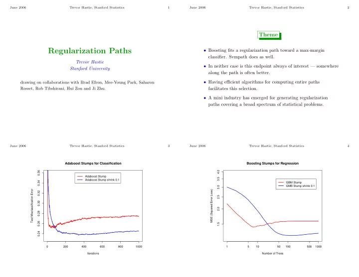
June 2006 Trevor Hastie, Stanford Statistics 1 June 2006 Trevor Hastie, Stanford Statistics 2 Theme Regularization Paths • Boosting fits a regularization path toward a max-margin classifier. Svmpath does as well. Trevor Hastie • In neither case is this endpoint always of interest — somewhere Stanford University along the path is often better. • Having efficient algorithms for computing entire paths drawing on collaborations with Brad Efron, Mee-Young Park, Saharon Rosset, Rob Tibshirani, Hui Zou and Ji Zhu. facilitates this selection. • A mini industry has emerged for generating regularization paths covering a broad spectrum of statistical problems. June 2006 Trevor Hastie, Stanford Statistics 3 June 2006 Trevor Hastie, Stanford Statistics 4 Adaboost Stumps for Classification Boosting Stumps for Regression 4.0 0.36 Adaboost Stump 3.5 Adaboost Stump shrink 0.1 0.34 GBM Stump GMB Stump shrink 0.1 3.0 Test Misclassification Error MSE (Squared Error Loss) 0.32 2.5 0.30 2.0 0.28 0.26 1.5 0.24 0 200 400 600 800 1000 1 5 10 50 100 500 1000 Iterations Number of Trees

June 2006 Trevor Hastie, Stanford Statistics 5 June 2006 Trevor Hastie, Stanford Statistics 6 Linear Regression Least Squares Boosting Here is a version of least squares boosting for multiple linear regression: (assume predictors are standardized) Friedman, Hastie & Tibshirani — see Elements of Statistical (Incremental) Forward Stagewise Learning (chapter 10) Supervised learning: Response y , predictors x = ( x 1 , x 2 . . . x p ). 1. Start with r = y , β 1 , β 2 , . . . β p = 0. 2. Find the predictor x j most correlated with r 1. Start with function F ( x ) = 0 and residual r = y 3. Update β j ← β j + δ j , where δ j = ǫ · sign � r, x j � 2. Fit a CART regression tree to r giving f ( x ) 4. Set r ← r − δ j · x j and repeat steps 2 and 3 many times 3. Set F ( x ) ← F ( x ) + ǫf ( x ), r ← r − ǫf ( x ) and repeat steps 2 and 3 many times δ j = � r, x j � gives usual forward stagewise; different from forward stepwise Analogous to least squares boosting, with trees=predictors June 2006 Trevor Hastie, Stanford Statistics 7 June 2006 Trevor Hastie, Stanford Statistics 8 Example: Prostate Cancer Data Linear regression via the Lasso (Tibshirani, 1995) Lasso Forward Stagewise lcavol lcavol • Assume ¯ y = 0, ¯ x j = 0, Var( x j ) = 1 for all j . 0.6 0.6 j x ij β j ) 2 subject to || β || 1 ≤ t • Minimize � i ( y i − � 0.4 0.4 • Similar to ridge regression , which has constraint || β || 2 ≤ t Coefficients Coefficients svi svi lweight lweight • Lasso does variable selection and shrinkage, while ridge only pgg45 pgg45 0.2 lbph 0.2 lbph shrinks. 0.0 0.0 gleason gleason β β 2 ^ . ^ . 2 β β age age -0.2 -0.2 lcp lcp β 1 β 1 0.0 0.5 1.0 1.5 2.0 2.5 0 50 100 150 200 250 t = P j | β j | Iteration

June 2006 Trevor Hastie, Stanford Statistics 9 June 2006 Trevor Hastie, Stanford Statistics 10 Diabetes Data Why are Forward Stagewise and Lasso so similar? Lasso Stagewise 9 9 500 500 • Are they identical? 3 3 6 6 4 4 • In orthogonal predictor case: yes 8 8 7 7 10 10 • In hard to verify case of monotone coefficient paths: yes • • • • • • • • • • • • • • • • • • • • 0 0 1 1 3 9 4 7 2 10 5 8 6 1 3 9 4 7 2 10 5 8 1 6 β j ˆ • In general, almost! 2 2 -500 -500 • Least angle regression (LAR) provides answers to these questions, and an efficient way to compute the complete Lasso 5 5 sequence of solutions. 0 1000 2000 3000 0 1000 2000 3000 t = P | ˆ t = P | ˆ β j | → β j | → June 2006 Trevor Hastie, Stanford Statistics 11 June 2006 Trevor Hastie, Stanford Statistics 18 Least Angle Regression — LAR LAR 0 2 3 4 5 7 8 10 f for LAR Like a “more democratic” version of forward stepwise regression. d 9 1. Start with r = y , ˆ β 1 , ˆ β 2 , . . . ˆ β p = 0. Assume x j standardized. 500 6 • d f are labeled at the 2. Find predictor x j most correlated with r . 4 Standardized Coefficients top of the figure 8 3. Increase β j in the direction of sign(corr( r, x j )) until some 10 • At the point a com- 0 1 other competitor x k has as much correlation with current petitor enters the ac- residual as does x j . 2 tive set, the d f are in- 4. Move (ˆ β j , ˆ β k ) in the joint least squares direction for ( x j , x k ) cremented by 1. −500 until some other competitor x ℓ has as much correlation with • Not true, for example, the current residual 5 for stepwise regression. 5. Continue in this way until all predictors have been entered. 0.0 0.2 0.4 0.6 0.8 1.0 |beta|/max|beta| Stop when corr( r, x j ) = 0 ∀ j , i.e. OLS solution.

✬ ✩ March 2003 Trevor Hastie, Stanford Statistics 14 June 2006 Trevor Hastie, Stanford Statistics 12 LARS x 2 x 2 20000 • 9 3 9 9 • 500 3 6 15000 4 8 ˆ 4 C k 7 10 8 7 10 10000 • • • • • • • • • • c kj | ¯ y 2 0 4 1 3 9 4 7 2 10 5 8 6 1 • β j ˆ | ˆ 7 2 5 • 1 u 2 5000 6 -500 2 y 1 ¯ • 10 ˆ • 5 µ 0 ˆ x 1 • µ 1 2 8 6 1 • • • 5 0 The LAR direction u 2 at step 2 makes an equal angle with x 1 and 0 1000 2000 3000 2 4 6 8 10 � | ˆ β j | → Step k → x 2 . ✫ ✪ June 2006 Trevor Hastie, Stanford Statistics 13 June 2006 Trevor Hastie, Stanford Statistics 14 Relationship between the 3 algorithms • Lasso and forward stagewise can be thought of as restricted versions of LAR • Forward Stagewise: Compute the LAR direction, but constrain • Lasso : Start with LAR. If a coefficient crosses zero, stop. Drop the sign of the coefficients to match the correlations corr( r, x j ). that predictor, recompute the best direction and continue. This • The incremental forward stagewise procedure approximates gives the Lasso path these steps, one predictor at a time. As step size ǫ → 0, can Proof: use KKT conditions for appropriate Lagrangian. Informally: show that it coincides with this modified version of LAR ∂ � 1 � 2 || y − X β || 2 � + λ | β j | = 0 ∂β j j ⇔ λ · sign( ˆ if ˆ � x j , r � = β j ) β j � = 0 (active)

June 2006 Trevor Hastie, Stanford Statistics 15 Data Mining Trevor Hastie, Stanford University 24 Cross-Validation Error Curve • 10-fold CV error curve using lasso on some diabetes data lars package (64 inputs, 442 samples). 6000 • Thick curve is CV error curve 5500 • The LARS algorithm computes the entire Lasso/FS/LAR path • Shaded region indicates stan- 5000 in same order of computation as one full least squares fit. CV Error dard error of CV estimate. 4500 • When p ≫ N , the solution has at most N non-zero coefficients. • Curve shows effect of over- 4000 Works efficiently for micro-array data ( p in thousands). fitting — errors start to in- 3500 • Cross-validation is quick and easy. crease above s = 0 . 2. 3000 • This shows a trade-off be- tween bias and variance. 0.0 0.2 0.4 0.6 0.8 1.0 Tuning Parameter s June 2006 Trevor Hastie, Stanford Statistics 16 June 2006 Trevor Hastie, Stanford Statistics 17 Forward Stagewise and the Monotone Lasso Degrees of Freedom of Lasso • Expand the variable set to in- Lasso Coefficients (Positive) clude their negative versions 4 3 − x j . • The d f or effective number of parameters give us an indication 2 1 of how much fitting we have done. 0 • Original lasso corresponds to Coefficients (Negative) 4 a positive lasso in this en- 3 Stein’s Lemma: If y i are i.i.d. N ( µ i , σ 2 ), • 2 larged space. 1 � n n � 0 ∂ ˆ µ i µ i , y i ) /σ 2 = E def � � • Forward stagewise corre- d f (ˆ µ ) = cov(ˆ Forward Stagewise ∂y i Coefficients (Positive) 4 sponds to a monotone lasso . i =1 i =1 3 The L 1 norm || β || 1 in this 2 • Degrees of freedom formula for LAR: After k steps, d f (ˆ µ k ) = k 1 enlarged space is arc-length . 0 exactly (amazing! with some regularity conditions) Coefficients (Negative) 4 3 • Forward stagewise produces • Degrees of freedom formula for lasso: Let ˆ d f (ˆ µ λ ) be the 2 1 the maximum decrease in loss number of non-zero elements in ˆ β λ . Then E ˆ d f (ˆ µ λ ) = d f (ˆ µ λ ). 0 per unit arc-length in coeffi- 0 20 40 60 80 L1 Norm (Standardized) cients.