In System Identification, System Identification: . . . Interval - PowerPoint PPT Presentation

System Identification: . . . Need to Take . . . How Can We Describe . . . Two Approximations, . . . In System Identification, System Identification: . . . Interval (and Fuzzy) Estimates Algorithm for the . . . Can Lead to Much Better Accuracy What if We . . . than the Traditional Statistical Ones: Simplest Case: Linear . . . General Algorithm and Case Study Results of Our Analysis Home Page Sergey I. Kumkov 1 , Vladik Kreinovich 2 , Andrzej Pownuk 2 Title Page ◭◭ ◮◮ 1 Institute of Mathematics and Mechanics, Ural Branch Russian Academy of Sciences, and Ural Federal University ◭ ◮ Ekaterinburg, Russia, kumkov@imm.uran.ru 2 Computational Science Program, University of Texas at El Paso Page 1 of 25 El Paso, TX 79968, USA, ampownuk@utep.edu, vladik@utep.edu Go Back Full Screen Close Quit

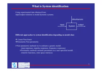
System Identification: . . . Need to Take . . . 1. System Identification: A General Problem How Can We Describe . . . • Often, we are interested in a quantity y which is diffi- Two Approximations, . . . cult (or even impossible) to measure directly. System Identification: . . . Algorithm for the . . . • This difficulty and/or impossibility may be technical: What if We . . . – while we can directly measure the distance between Simplest Case: Linear . . . the two buildings by simply walking there, Results of Our Analysis – there is no easy way to measure the distance to a Home Page nearby star by flying there. Title Page • Impossibility may come from predictions – today, we ◭◭ ◮◮ cannot measure tomorrow’s temperature. ◭ ◮ Page 2 of 25 Go Back Full Screen Close Quit

System Identification: . . . Need to Take . . . 2. System Identification (cont-d) How Can We Describe . . . • A natural idea is to find easier-to-measure quantities Two Approximations, . . . x 1 , . . . , x n that are related to y by a known dependence System Identification: . . . Algorithm for the . . . y = f ( x 1 , . . . , x n ) . What if We . . . • Then, we can use the results � x i of measuring these Simplest Case: Linear . . . def auxiliary quantities to estimate y as � = f ( � x 1 , . . . , � x n ). y Results of Our Analysis Home Page • Example: we can find the distance to a nearby star by Title Page measuring the direction to this star in two seasons: ◭◭ ◮◮ – when the Earth is at different sides of the Sun, and ◭ ◮ – the angle is thus slightly different. Page 3 of 25 • To predict tomorrow’s temperature T : Go Back – we can measure the temperature and wind speed and direction at different locations today, and Full Screen – use this data to predict T . Close Quit

System Identification: . . . Need to Take . . . 3. System Identification (final) How Can We Describe . . . • In some cases, we know the dependence Two Approximations, . . . System Identification: . . . y = f ( x 1 , . . . , x n ) . Algorithm for the . . . What if We . . . • In other cases, we only know the general form of this Simplest Case: Linear . . . dependence Results of Our Analysis y = f ( a 1 , . . . , a m , x 1 , . . . , x n ) . Home Page Title Page • The values a i must be estimated based on measurement results. ◭◭ ◮◮ • We have the results � y k and � x ki of measuring y and x i ◭ ◮ in several situations k = 1 , . . . , K . Page 4 of 25 • Estimating a i is called system identification . Go Back Full Screen Close Quit

System Identification: . . . Need to Take . . . 4. Need to Take Measurement Uncertainty into How Can We Describe . . . Account Two Approximations, . . . • Measurements are not 100% accurate. System Identification: . . . Algorithm for the . . . • In general, the measurement result � x is different from What if We . . . def the actual (unknown) value x : ∆ x = � x − x � = 0; thus, Simplest Case: Linear . . . – while for the (unknown) actual values y k and x ki , Results of Our Analysis we have y k = f ( a 1 , . . . , a m , x k 1 , . . . , x kn ) , Home Page y k ≈ y k – the relation between measurement results � Title Page x ki ≈ x ki is approximate: and � ◭◭ ◮◮ y k ≈ f ( a 1 , . . . , a m , � � x k 1 , . . . , � x kn ) . ◭ ◮ • It is therefore important to take this uncertainty into Page 5 of 25 account when estimating the values a 1 , . . . , a m . Go Back Full Screen Close Quit

System Identification: . . . Need to Take . . . 5. How Can We Describe Uncertainty? How Can We Describe . . . • In all the cases, we should know the bound ∆ on the Two Approximations, . . . absolute value of the measurement error: | ∆ x | ≤ ∆. System Identification: . . . Algorithm for the . . . • This means that only values ∆ x from the interval What if We . . . [ − ∆ , ∆] are possible. Simplest Case: Linear . . . • If this is the only information we have then: Results of Our Analysis Home Page – based on the measurement result � x , – the only information that we have about the actual Title Page value x is that x ∈ [ � x − ∆ , � x + ∆]. ◭◭ ◮◮ • Processing data under such interval uncertainty is ◭ ◮ known as interval computations . Page 6 of 25 Go Back Full Screen Close Quit

System Identification: . . . Need to Take . . . 6. How Can We Describe Uncertainty (cont-d) How Can We Describe . . . • Ideally, it is also desirable to know how frequent are Two Approximations, . . . different values ∆ x within this interval. System Identification: . . . Algorithm for the . . . • In other words, it is desirable to know the probabilities What if We . . . of different values ∆ x ∈ [ − ∆ , ∆]. Simplest Case: Linear . . . • The measurement uncertainty ∆ x often comes from Results of Our Analysis many different independent sources. Home Page • Thus, due to the Central Limit Theorem, the distribu- Title Page tion of ∆ x is close to Gaussian. ◭◭ ◮◮ • This explains the usual engineering practice of using ◭ ◮ normal distributions. Page 7 of 25 Go Back Full Screen Close Quit

System Identification: . . . Need to Take . . . 7. Two Approximations, Two Options How Can We Describe . . . • Gaussian distribution is that it is not located on any Two Approximations, . . . interval. System Identification: . . . Algorithm for the . . . • The probability of measurement error ∆ x to be in any What if We . . . interval – no matter how far away from ∆ – is non-zero. Simplest Case: Linear . . . • From this viewpoint, the assumption that the distribu- Results of Our Analysis tion is Gaussian is an approximation. Home Page • It seems like a very good approximation, since for nor- Title Page mal distribution with mean 0 and st. dev. σ : ◭◭ ◮◮ – the probability to be outside the 3 σ interval ◭ ◮ [ − 3 σ, 3 σ ] is very small, approximately 0.1%, and Page 8 of 25 – the probability for it to be outside the 6 σ interval is about 10 − 8 , practically negligible. Go Back Full Screen • Since the difference is small, this should not affect sys- tem identification. Close Quit

System Identification: . . . Need to Take . . . 8. Two Approximations, Two Options (cont-d) How Can We Describe . . . • At first glance, if we keep the bounds but ignore prob- Two Approximations, . . . abilities, we will do much worse. System Identification: . . . Algorithm for the . . . • Our results show that the opposite is true: What if We . . . – if we ignore the probabilistic information and use Simplest Case: Linear . . . only interval (or fuzzy) information, Results of Our Analysis – we get much more accurate estimates for a j than Home Page in the statistical case. Title Page • This is not fully surprising: theory shows that asymp- ◭◭ ◮◮ totically, interval bounds are better. ◭ ◮ • However, the drastic improvement in accuracy was Page 9 of 25 somewhat unexpected. Go Back Full Screen Close Quit

System Identification: . . . Need to Take . . . 9. System Identification: Interval Case How Can We Describe . . . • For each pattern k = 1 , . . . , K : Two Approximations, . . . System Identification: . . . – we know the measurement results � y k and � x ki , and Algorithm for the . . . – we know the accuracies ∆ k and ∆ ki of the corre- What if We . . . sponding measurements. Simplest Case: Linear . . . • Thus, we know that: Results of Our Analysis – the actual (unknown) value y k belongs to the inter- Home Page val [ y k , y k ] = [ � y k − ∆ k , � y k + ∆ k ]; and Title Page – the actual (unknown) value x ki belongs to the in- ◭◭ ◮◮ terval [ x ki , x ki ] = [ � x ki − ∆ ki , � x ki + ∆ ki ] . ◭ ◮ • We need to find a 1 , . . . , a m for which, for every k , for some x ki ∈ [ x ki , x ki ], Page 10 of 25 f ( a 1 , . . . , a m , x k 1 , . . . , x kn ) ∈ [ y k , y k ] . Go Back Full Screen • Specifically, for each j from 1 to m , we would like to find the range [ a j , a j ] of all possible values of a j . Close Quit