Outlier Outlier Outlier- Outlier - -robust - robust robust - PowerPoint PPT Presentation
GESG seminar, 16 October 2015, UFM Outlier Outlier Outlier- Outlier - -robust - robust robust robust identification identification identification of identification of of of switching regimes: switching regimes: switching regimes:
GESG seminar, 16 October 2015, UFM Outlier Outlier Outlier- Outlier - -robust - robust robust robust identification identification identification of identification of of of switching regimes: switching regimes: switching regimes: switching regimes: an application to an application to an application to an application to the S&P the S&P the S&P 500 the S&P 500 500 500 ������������������������������������������ ���������� ������������� ���������������������������������
S&P 500 1990 to 2015 (C) SZABOLCS BLAZSEK 2
S&P 500 1990 to 2015 (C) SZABOLCS BLAZSEK 3
Markov regime Markov regime Markov regime Markov regime- - - -switching models switching models switching models switching models In financial markets, high and low volatility periods switch each other. The class of Markov regime-switching (MS) models (Hamilton, 1989; Kim and Nelson, 1999) is a possible way of modelling the time-varying probability distribution of asset returns. MS models assume that data are generated by a mixture of different probability distributions with time-varying parameters which are driven by an underlying Markov chain. (C) SZABOLCS BLAZSEK 4
Objective of paper, Outliers Objective of paper, Outliers Objective of paper, Outliers Objective of paper, Outliers The main objective is to study the performance of different dynamic two-state MS models for which the treatment of outliers is different . “An outlier is an observation which is inconsistent with a model which is thought to be appropriate for the overwhelming majority of the observations” (Harvey, 1989). For a two-state MS model, outliers are not generated by any of the regimes. (C) SZABOLCS BLAZSEK 5
Idea Idea Idea Idea Suppose that the initial observations of the sample are generated by the low volatility regime. When the first observation of the high volatility regime arrives, then it will be an outlier for the low volatility regime. If this observation is followed by subsequent volatile observations, then the MS model will recognize that the process has entered the high volatility regime, and the high volatility observation no longer is an outlier. (C) SZABOLCS BLAZSEK 6
Idea Idea Idea Idea Nevertheless, from time to time, such extreme observations appear that do not belong to any of the regimes. The question is how effectively a two-regime dynamic regime-switching model can identify the switch between different regimes in these cases. We show that this crucially depends on how outlier observations are treated by the dynamic model. (C) SZABOLCS BLAZSEK 7
Idea Idea Idea Idea We consider two dynamic models for asset return volatility: First, the well-known generalized autoregressive conditional heteroscedasticity (GARCH) model (Bollerslev, 1986; Taylor, 1986). Second, the recent and from a statistical point of view very effective Beta-t-EGARCH model (Harvey and Chakravarty, 2008) that belongs to class of dynamic conditional score (DCS) models (Harvey, 2013). (C) SZABOLCS BLAZSEK 8
Idea Idea Idea Idea - - - - GARCH GARCH GARCH GARCH In GARCH the dynamic equation is updated by the square of the previous observation in each time period. Thus, GARCH accentuates outliers in the conditional variance equation . If GARCH is persistent, then outliers will impact future observations through the conditional variance. Therefore, the regime-switching GARCH model can be rather confused by outlier observations which are not generated by any of the regimes. (C) SZABOLCS BLAZSEK 9
Idea Idea Idea Idea - - - - DCS DCS DCS DCS In DCS models the dynamic equation is updated by lags of the conditional score with respect to a time-dependent parameter. An important property of these models is that the conditional score discounts extreme observations . Therefore, in DCS models outliers will have little effect on future observations . Hence, a regime-switching DCS model is not sensitive to outliers and it may identify different regimes effectively. (C) SZABOLCS BLAZSEK 10
Data Data Data Data Daily percentage change in S&P 500 for period 2 January 1990 to 17 June 2015 T =6,416 days are observed ( source : Bloomberg) (C) SZABOLCS BLAZSEK 11
MS MS- -ARMA(1,1) plus MS ARMA(1,1) plus MS- -GARCH(1,1) GARCH(1,1) MS MS - - ARMA(1,1) plus MS ARMA(1,1) plus MS - - GARCH(1,1) GARCH(1,1) with leverage effects with leverage effects with leverage effects with leverage effects Location (MS-ARMA): (C) SZABOLCS BLAZSEK 12
MS MS- -ARMA(1,1) plus MS ARMA(1,1) plus MS- -GARCH(1,1) GARCH(1,1) MS MS - - ARMA(1,1) plus MS ARMA(1,1) plus MS - - GARCH(1,1) GARCH(1,1) with with with with leverage effects leverage effects leverage effects leverage effects In the location, we avoid path-dependence by Scale (MS-GARCH with leverage effects): (C) SZABOLCS BLAZSEK 13
MS MS- -ARMA(1,1) plus MS ARMA(1,1) plus MS- -GARCH(1,1) GARCH(1,1) MS MS - - ARMA(1,1) plus MS ARMA(1,1) plus MS - - GARCH(1,1) GARCH(1,1) with with with with leverage effects leverage effects leverage effects leverage effects (C) SZABOLCS BLAZSEK 14
Why to include leverage effects? Why to include leverage effects? Why to include leverage effects? Why to include leverage effects? “Volatility tends to respond more to falls in stock prices than to rises. One explanation for this phenomenon is that a drop in the share price of a firm will lower the market value and thereby increase the debt-equity ratio. As a result, the risk to investors, as residual claimants, is increased. Hence the term leverage effect” (Harvey, 2013). (C) SZABOLCS BLAZSEK 15
MS MS- -QAR(1) plus MS QAR(1) plus MS- -Beta Beta- -t t- -EGARCH(1,1) EGARCH(1,1) MS MS - - QAR(1) plus MS QAR(1) plus MS - - Beta Beta - - t t - - EGARCH(1,1) EGARCH(1,1) with leverage effects with leverage effects with leverage effects with leverage effects (C) SZABOLCS BLAZSEK 16
Location (quasi-AR, QAR): (C) SZABOLCS BLAZSEK 17
(C) SZABOLCS BLAZSEK 18
Scale (Beta-t-EGARCH with leverage effects): (C) SZABOLCS BLAZSEK 19
(C) SZABOLCS BLAZSEK 20
Results Results Results Results We are not able to estimate MS-ARMA plus MS-GARCH with leverage effects. Some parameters converge to the boundary of the parameter space in the numerical maximization of the log likelihood function. MS-QAR plus MS-Beta-t-EGARCH with leverage effects can be estimated very effectively. The ML estimation procedure is robust. For MS-QAR plus MS-Beta-t-EGARCH with leverage effects we have the next filtered probability series: (C) SZABOLCS BLAZSEK 21
Filtered probabilities of the high volatility regime (C) SZABOLCS BLAZSEK 22
Results Results Results Results The main difference between the benchmark regime- switching model and the MS-DCS model considered is the way in which observations are transformed in the innovation term of conditional location and scale equations . The failure of MS-ARMA plus MS-t-GARCH with leverage effects and the success of MS-QAR plus MS-Beta-t-EGARCH with leverage effects supports the main point of this work, outlined in the introduction. (C) SZABOLCS BLAZSEK 23
Results Results Results Results We compared the full model, MS-QAR plus MS-Beta-t- EGARCH with leverage effects with: a) MS-QAR plus MS-Beta-t-EGARCH without leverage effects b) QAR plus Beta-t-EGARCH with leverage effects c) QAR plus Beta-t-EGARCH without leverage effects (C) SZABOLCS BLAZSEK 24
Results Results Results Results The MS-QAR plus MS-Beta-t-EGARCH with leverage effects is superior to all alternatives with respect to LL, AIC, BIC and HQC. The leverage effects coefficient is highly significant in MS- QAR plus MS-Beta-t-EGARCH with leverage effects. Conditions of covariance stationarity (Abramson and Cohen, 2007) hold for MS-QAR plus MS-Beta-t-EGARCH with leverage effects. (C) SZABOLCS BLAZSEK 25
Thank you for your attention! SBLAZSEK@UFM.EDU SBLAZSEK@UFM.EDU SBLAZSEK@UFM.EDU SBLAZSEK@UFM.EDU (C) SZABOLCS BLAZSEK 26
Abramson, A. and Cohen, I. (2007) On the stationarity of Markov switching GARCH processes, Econometric Theory , 23. Bollerslev, T. (1986) Generalized autoregressive conditional heteroskedasticity, Journal of Econometrics , 31. Hamilton, J. D. (1989) A new approach to the economic analysis of nonstationary time series and the business cycle, Econometrica , 57. Harvey, A. C. (1989) Forecasting, Structural Time Series Models and the Kalman Filter , Cambridge University Press. Harvey, A. C. (2013) Dynamic Models for Volatility and Heavy Tails , Cambridge University Press. Harvey, A. C. and Chakravarty, T. (2008) Beta-t-(E)GARCH. Cambridge Working Papers in Economics 0840, Faculty of Economics, University of Cambridge. Kim, C. J. and Nelson, C. R. (1999) State-Space Models with Regime Switching , MIT Press. Taylor, S. J. (1986) Modelling financial time series , Wiley. (C) SZABOLCS BLAZSEK 27
Recommend
More recommend
Explore More Topics
Stay informed with curated content and fresh updates.
