Overview IAML: Linear Regression The linear model Fitting the - PowerPoint PPT Presentation
Overview IAML: Linear Regression The linear model Fitting the linear model to data Probabilistic interpretation of the error function Nigel Goddard School of Informatics Examples of regression problems Dealing with multiple
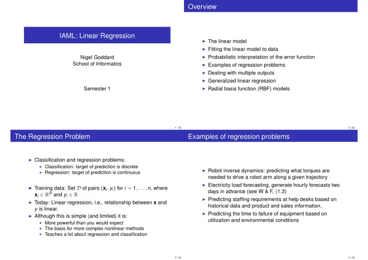
Overview IAML: Linear Regression ◮ The linear model ◮ Fitting the linear model to data ◮ Probabilistic interpretation of the error function Nigel Goddard School of Informatics ◮ Examples of regression problems ◮ Dealing with multiple outputs ◮ Generalized linear regression ◮ Radial basis function (RBF) models Semester 1 1 / 38 2 / 38 The Regression Problem Examples of regression problems ◮ Classification and regression problems: ◮ Classification: target of prediction is discrete ◮ Robot inverse dynamics: predicting what torques are ◮ Regression: target of prediction is continuous needed to drive a robot arm along a given trajectory ◮ Electricity load forecasting, generate hourly forecasts two ◮ Training data: Set D of pairs ( x i , y i ) for i = 1 , . . . , n , where ◮ days in advance (see W & F, § 1.3) x i ∈ R D and y i ∈ R ◮ Predicting staffing requirements at help desks based on ◮ Today: Linear regression, i.e., relationship between x and historical data and product and sales information, y is linear. ◮ Predicting the time to failure of equipment based on ◮ Although this is simple (and limited) it is: utilization and environmental conditions ◮ More powerful than you would expect ◮ The basis for more complex nonlinear methods ◮ Teaches a lot about regression and classification 3 / 38 4 / 38
The Linear Model Toy example: Data ◮ Linear model 4 ● ● 3 ● f ( x ; w ) = w 0 + w 1 x 1 + . . . + w D x D ● ● ● ● = φ ( x ) w 2 ● ● ● ● ● ● ● ● y 1 ● where φ ( x ) = ( 1 , x 1 , . . . , x D ) = ( 1 , x T ) ● ● ● ● and 0 ● w 0 ● ● −1 ● ● w 1 w = (1) −2 ... w D −3 −2 −1 0 1 2 3 ◮ The maths of fitting linear models to data is easy. We use x the notation φ ( x ) to make generalisation easy later. 5 / 38 6 / 38 Toy example: Data With two features Y 4 4 ● ● ● ● 3 3 ● ● • • ● ● ● ● ● ● ● ● • • • • • • 2 ● 2 ● • • • • ● ● ● ● • • • ● ● ● ● • • • ● ● ● ● • • • • • • • ● ● • • y 1 y 1 • • • • ● ● • • • • • • • • • • • • • • ● ● ● ● ● ● ● ● • • 0 0 • • • • • • ● ● • • • • • • • • • • • ● ● ● ● • −1 −1 ● ● ● ● • • • • • • X 2 −2 −2 • • • −3 −2 −1 0 1 2 3 −3 −2 −1 0 1 2 3 X 1 x x Instead of a line, a plane . With more features, a hyperplane . Figure: Hastie, Tibshirani, and Friedman 7 / 38 8 / 38
With more features With more features CPU Performance Data Set ◮ Predict: PRP: published relative performance PRP = - 56.1 + 0.049 MYCT ◮ MYCT: machine cycle time in nanoseconds (integer) + 0.015 MMIN ◮ MMIN: minimum main memory in kilobytes (integer) + 0.006 MMAX ◮ MMAX: maximum main memory in kilobytes (integer) + 0.630 CACH ◮ CACH: cache memory in kilobytes (integer) - 0.270 CHMIN ◮ CHMIN: minimum channels in units (integer) + 1.46 CHMAX ◮ CHMAX: maximum channels in units (integer) 9 / 38 10 / 38 In matrix notation Linear Algebra: The 1-Slide Version What is matrix multiplication? a 11 a 12 a 13 b 1 , b = A = a 21 a 22 a 23 b 2 ◮ Design matrix is n × ( D + 1 ) a 31 a 32 a 33 b 3 1 x 11 x 12 . . . x 1 D First consider matrix times vector, i.e., A b . Two answers: 1 x 21 x 22 . . . x 2 D Φ = . . . . . . . . . . 1. A b is a linear combination of the columns of A . . . . . 1 x n 1 x n 2 . . . x nD a 11 a 12 a 13 + b 2 + b 3 Ab = b 1 a 21 a 22 a 23 ◮ x ij is the j th component of the training input x i a 31 a 32 a 33 ◮ Let y = ( y 1 , . . . , y n ) T 2. A b is a vector. Each element of the vector is the dot ◮ Then ˆ y = Φ w is ...? products between b and one row of A . ( a 11 , a 12 , a 13 ) b A b = ( a 21 , a 22 , a 23 ) b ( a 31 , a 32 , a 33 ) b 11 / 38 12 / 38
Linear model (part 2) Solving for Model Parameters This looks like what we’ve seen in linear algebra In matrix notation: y = Φ w ◮ Design matrix is n × ( D + 1 ) We know y and Φ but not w . . . . 1 x 11 x 12 x 1 D 1 x 21 x 22 . . . x 2 D Φ = . . . . . So why not take w = Φ − 1 y ? (You can’t, but why?) . . . . . . . . . . 1 x n 1 x n 2 . . . x nD ◮ x ij is the j th component of the training input x i ◮ Let y = ( y 1 , . . . , y n ) T ◮ Then ˆ y = Φ w is the model’s predicted values on training inputs. 13 / 38 14 / 38 Solving for Model Parameters Loss function This looks like what we’ve seen in linear algebra y = Φ w Want a loss function O ( w ) that We know y and Φ but not w . ◮ We minimize wrt w . ◮ At minimum, ˆ y looks like y . So why not take w = Φ − 1 y ? (You can’t, but why?) ◮ (Recall: ˆ y depends on w ) Three reasons: ˆ y = Φ w ◮ Φ is not square. It is n × ( D + 1 ) . ◮ The system is overconstrained ( n equations for D + 1 parameters), in other words ◮ The data has noise 15 / 38 16 / 38
Fitting a linear model to data Fitting a linear model to data ◮ n � ( y i − w T x i ) 2 O ( w ) = Y i = 1 ◮ A common choice: squared error = ( y − Φ w ) T ( y − Φ w ) (makes the maths easy) ◮ We want to minimize this with respect to w . • • • • • • • • n • • ◮ The error surface is a parabolic bowl • • • • • • � ( y i − w T x i ) 2 • • O ( w ) = • • • • • • • • • 25 • • • • • • • • • • • • • • • • i = 1 • • 20 • • • • • • • • • • • • • • 15 • • ◮ In the picture: this is sum of • • • • E[w] • • 10 • • squared length of black sticks. • • X 2 • 5 ◮ (Each one is called a residual , • 0 • i.e., each y i − w T x i ) 2 X 1 1 -2 -1 0 0 1 2 -1 3 w1 w0 ◮ How do we do this? 17 / 38 18 / 38 The Solution Probabilistic interpretation of O ( w ) ◮ Assume that y = w T x + ǫ , where ǫ ∼ N ( 0 , σ 2 ) ◮ Answer: to minimize O ( w ) = � n i = 1 ( y i − w T x i ) 2 , set partial ◮ (This is an exact linear relationship plus Gaussian noise.) derivatives to 0. ◮ This implies that y | x i ∼ N ( w T x i , σ 2 ) , i.e. ◮ This has an analytical solution √ 2 π + log σ + ( y i − w T x i ) 2 w = (Φ T Φ) − 1 Φ T y − log p ( y i | x i ) = log ˆ 2 σ 2 ◮ (Φ T Φ) − 1 Φ T is the pseudo-inverse of Φ ◮ So minimising O ( w ) equivalent to maximising likelihood! ◮ First check: Does this make sense? Do the matrix ◮ Can view w T x as E [ y | x ] . dimensions line up? ◮ Squared residuals allow estimation of σ 2 ◮ Then: Why is this called a pseudo-inverse? () n σ 2 = 1 ◮ Finally: What happens if there are no features? � ( y i − w T x i ) 2 ˆ n i = 1 19 / 38 20 / 38
Sensitivity to Outliers ◮ Linear regression is sensitive to outliers √ ◮ Example: Suppose y = 0 . 5 x + ǫ , where ǫ ∼ N ( 0 , 0 . 25 ) , Fitting this into the general structure for learning algorithms: and then add a point (2.5,3): 3.0 ● ◮ Define the task : regression ◮ Decide on the model structure : linear regression model 2.5 ◮ Decide on the score function : squared error (likelihood) ● ● 2.0 ◮ Decide on optimization/search method to optimize the score function: calculus (analytic solution) 1.5 ● 1.0 ● 0.5 ● 0.0 0 1 2 3 4 5 21 / 38 22 / 38 Diagnositics Dealing with multiple outputs Graphical diagnostics can be useful for checking: ◮ Is the relationship obviously nonlinear? Look for structure ◮ Suppose there are q different targets for each input x in residuals? ◮ Are there obvious outliers? ◮ We introduce a different w i for each target dimension, and do regression separately for each one The goal isn’t to find all problems. You can’t. The goal is to find ◮ This is called multiple regression obvious, embarrassing problems. Examples: Plot residuals by fitted values. Stats packages will do this for you. 23 / 38 24 / 38
Recommend
More recommend
Explore More Topics
Stay informed with curated content and fresh updates.
