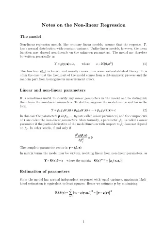
LINEAR REGRESSION LINEAR REGRESSION - FROM A MACHINE LEARNING POINT - PowerPoint PPT Presentation

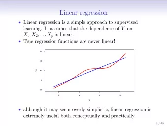
LINEAR REGRESSION

LINEAR REGRESSION - FROM A MACHINE LEARNING POINT OF VIEW 25 SIMPLE LINEAR REGRESSION 20 Sales 15 ▸ Starting point 10 ▸ Simplest parametric function 5 ▸ Easy to interpret the parameters: 0 50 100 150 200 250 300 intercept, coefficients: unit change in x TV makes coefficient times unit change in y Y ≈ β 0 + β 1 X. Y = β 0 + β 1 X + � . ▸ Can be very accurate in certain problems sales ≈ β 0 + β 1 × TV . ▸ Least squares N � 1 � 2 � � � � 1 � y i � y.x i / � Y P. data j model / /  y exp ▸ Insight: minimising (log) probability 2 � i D 0 (actually the likelihood) of observations given Gaussian y distribution � n i =1 ( x i − ¯ x )( y i − ¯ y ) ˆ β 1 = , � n i =1 ( x i − ¯ x ) 2 ˆ y − ˆ β 0 = ¯ β 1 ¯ x, �

LINEAR REGRESSION - FROM A MACHINE LEARNING POINT OF VIEW 10 10 ACCURACY OF COEFFICIENTS 5 5 Y Y 0 0 − 5 − 5 ▸ Data is from a true relationship + errors − 10 − 10 ▸ We get the line which fits the − 2 − 1 0 1 2 − 2 − 1 0 1 2 measurements most accurately using X X OLS Y = β 0 + β 1 X + � . RSS = e 2 1 + e 2 2 + · · · + e 2 n , ▸ The true and the measured coefficients will be different! � 1 � x 2 σ 2 2 = σ 2 ¯ 2 = SE(ˆ SE(ˆ � n � n β 0 ) n + , β 1 ) x ) 2 , i =1 ( x i − ¯ x ) 2 i =1 ( x i − ¯ ▸ We can estimate the standard errors of estimated parameters, ( assuming of σ is known as the re ˆ � β 1 − 0 uncorrelated errors which have a t = , RSE = RSS / ( n − 2). SE(ˆ β 1 ) � common variance (sigma) ) ▸ We can estimate the errors from the Coe ffi cient Std. error t-statistic p-value 7.0325 0.4578 15.36 < 0 . 0001 Intercept data itself: residual standard error, RSE 0.0475 0.0027 17.67 < 0 . 0001 TV

LINEAR REGRESSION - FROM A MACHINE LEARNING POINT OF VIEW 25 ACCURACY OF ESTIMATION 20 Sales 15 ▸ How accurate it the fit? 10 ▸ RSE, Residual standard errors 5 ▸ Closely related to chi-square 0 50 100 150 200 250 300 commonly used by physicist Y = β 0 + β 1 X + � . RSS = e 2 1 + e 2 2 + · · · + e 2 TV n , ▸ R squared, proportion of variance � n � � 1 1 � explained � RSE = n − 2RSS = ( y i − ˆ y i ) 2 . � n − 2 i =1 ▸ For simple linear regression R R 2 = TSS − RSS = 1 − RSS y ) 2 where TSS = � ( y i − ¯ squared is the same as Cor(x, y) TSS TSS .16). TSS measures th ▸ R is more general: multiple regression or nonlinear � n i =1 ( x i − x )( y i − y ) regression Cor( X, Y ) = i =1 ( y i − y ) 2 , �� n i =1 ( x i − x ) 2 �� n

LINEAR REGRESSION - FROM A MACHINE LEARNING POINT OF VIEW Sales MULTIPLE LINEAR REGRESSION ▸ Multiple x variables ▸ OLS TV ▸ Without other variables newspaper ads seem to be Radio related to sales, with other it does not Y = β 0 + β 1 X 1 + β 2 X 2 + · · · + β p X p + � , ▸ Ad spendings are Coe ffi cient Std. error t-statistic p-value correlated 9.312 0.563 16.54 < 0 . 0001 Intercept TV radio newspaper sales 0.203 0.020 9.92 < 0 . 0001 radio 1.0000 0.0548 0.0567 0.7822 TV ▸ Multiple regression 1.0000 0.3541 0.5762 radio Coe ffi cient Std. error t-statistic p-value 1.0000 0.2283 coefficients describe the newspaper 12.351 0.621 19.88 < 0 . 0001 Intercept 1.0000 sales effect of an input on the 0.055 0.017 3.30 0 . 00115 newspaper outcome given fixed other inputs Coe ffi cient Std. error t-statistic p-value ▸ Including all possible 2.939 0.3119 9.42 < 0 . 0001 Intercept factors can reveal the real 0.046 0.0014 32.81 < 0 . 0001 TV effect of variables 0.189 0.0086 21.89 < 0 . 0001 radio − 0.001 0.0059 − 0.18 0 . 8599 newspaper (adjusting for …)

LINEAR REGRESSION - FROM A MACHINE LEARNING POINT OF VIEW QUALITATIVE INPUTS TO LINEAR REGRESSION ▸ X can be a category ▸ Gender, ethnicity, marital status, phone type, country, .. � � 1 if i th person is female 1 if i th person is female ▸ Binary inputs x i = x i = − 1 if i th person is male 0 if i th person is male , � � 1 if i th person is Caucasian 1 if i th person is Asian x i 2 = x i 1 = ▸ Multiple categories 0 if i th person is not Asian , 0 if i th person is not Caucasian . ▸ It is called one-hot  β 0 + β 1 + � i if i th person is Asian   y i = β 0 + β 1 x i 1 + β 2 x i 2 + � i = β 0 + β 2 + � i if i th person is Caucasian encoding  β 0 + � i if i th person is African American . 

LINEAR REGRESSION - FROM A MACHINE LEARNING POINT OF VIEW Sales EXTENDING LINEAR REGRESSION: INTERACTIONS ▸ Linear regression is additive ▸ Best strategy? TV ▸ Spend all our money on radio ads Radio ▸ Some companies do that, but others have Coe ffi cient Std. error t-statistic p-value more balanced strategy 2.939 0.3119 9.42 < 0 . 0001 Intercept 0.046 0.0014 32.81 < 0 . 0001 TV 0.189 0.0086 21.89 < 0 . 0001 ▸ Interaction (synergy) between TV and radio radio − 0.001 0.0059 − 0.18 0 . 8599 newspaper ▸ TV x radio is just treated as a new variable, Y = β 0 + β 1 X 1 + β 2 X 2 + β 3 X 1 X 2 + � . OLS fitting as before Coe ffi cient Std. error t-statistic p-value 6.7502 0.248 27.23 < 0 . 0001 Intercept ▸ Y is not a linear function of X, but linear in 0.0191 0.002 12.70 < 0 . 0001 TV B-s, and the same formalism can be used 0.0289 0.009 3.24 0.0014 radio 0.0011 0.000 20.73 < 0 . 0001 TV × radio ▸ B_3 can be interpreted as the increase of the = β 0 + ( β 1 + β 3 X 2 ) X 1 + β 2 X 2 + � Y effectiveness of TV ads for one unit increase in radio ads = β 0 + β 1 × TV + β 2 × radio + β 3 × ( radio × TV ) + � × × × × sales β 0 + ( β 1 + β 3 × radio ) × TV + β 2 × radio + � .

LINEAR REGRESSION - FROM A MACHINE LEARNING POINT OF VIEW EXTENDING LINEAR REGRESSION: POLYNOMIAL REGRESSION 50 Linear Degree 2 Degree 5 ▸ Effects may be non linear, e.g.: very 40 often saturating Miles per gallon ▸ We can add polynomials of x as 30 different variables, OLS fitting as before 20 ▸ Again, y is not a linear function of x, 10 but linear in B-s, and the same 50 100 150 200 formalism can be used Horsepower mpg = β 0 + β 1 × horsepower + β 2 × horsepower 2 + � ▸ Actually we can use any functions of x, log(x), cos(x), sin(x), etc. Until the Coe ffi cient Std. error t-statistic p-value outcome is linear in the coefficients. 56.9001 1.8004 31.6 < 0 . 0001 Intercept − 0.4662 0.0311 − 15.0 < 0 . 0001 horsepower E.g.: we can not use cos(a*x+b) in horsepower 2 0.0012 0.0001 10.1 < 0 . 0001 linear regression.

LINEAR REGRESSION - FROM A MACHINE LEARNING POINT OF VIEW DETECTING NON-LINEARITY, OUTLIERS, HIGH LEVERAGE Residual Plot for Linear Fit Residual Plot for Quadratic Fit ▸ Clear trends in residuals indicate 20 323 334 15 323 non-linearity 15 330 334 10 10 ▸ Residuals plots are also useful to 5 Residuals Residuals 5 identify outliers 0 0 − 5 − 5 ▸ Could be just measurement − 10 − 10 error or indicate problems − 15 155 − 15 with the model itself 5 10 15 20 25 30 15 20 25 30 35 Fitted values Fitted values ▸ High leverage points have strong 20 20 20 6 6 effect on coefficients 4 Studentized Residuals 3 4 4 Residuals 2 2 Y 2 41 1 0 0 0 − 2 10 − 1 − 4 20 − 2 − 1 0 1 2 − 2 0 2 4 6 − 2 0 2 4 6 Y 5 X Fitted Values Fitted Values 0 x ) 2 h i = 1 ( x i − ¯ n + x ) 2 . � n i ′ =1 ( x i ′ − ¯ − 2 − 1 0 1 2 3 4 X

LINEAR REGRESSION - FROM A MACHINE LEARNING POINT OF VIEW 80 800 COLLINEARITY 70 600 60 Rating Age ▸ Some predictive variables can be 50 400 highly correlated 40 200 30 ▸ Their individual effect can not be 2000 4000 6000 8000 12000 2000 4000 6000 8000 12000 inferred Limit Limit 5 21.8 0 21.8 ▸ For 3 or more variables it is harder to 2 1 . 5 4 − 1 2 1 . 2 5 detect: multicollinearity 21.5 3 β Rating β Age − 2 2 − 3 ▸ Variance inflation factor, VIF 1 − 4 0 ▸ Possible solutions: drop one, or − 5 combine them? 0.16 0.17 0.18 0.19 − 0.1 0.0 0.1 0.2 β Limit β Limit Coe ffi cient Std. error t-statistic p-value − 173.411 43.828 − 3.957 < 0 . 0001 Intercept Model 1 − 2.292 0.672 − 3.407 0 . 0007 age 0.173 0.005 34.496 < 0 . 0001 limit − 377.537 45.254 − 8.343 < 0 . 0001 Intercept Model 2 2.202 0.952 2.312 0.0213 rating 0.025 0.064 0.384 0.7012 limit

LINEAR REGRESSION - FROM A MACHINE LEARNING POINT OF VIEW SOLVING MULTIPLE LINEAR ⎡ ⎤ N M 1 REGRESSION � � ⎦ X k ( x i ) 0 = a j X j ( x i ) k = 1 , . . . , M ⎣ y i − σ 2 i i =1 j =1 ▸ Linear regression can N y i X k ( x i ) � [ β ] = A T · b β k = usually be solved by σ 2 i i =1 matrix inversion N X j ( x i ) X k ( x i ) � α kj = [ α ] = A T · A σ 2 ▸ But sometimes normal i i =1 an matrix, and equations can be close M � A T · A · a = A T · b α kj a j = β k � � to singular, and it fails j =1 � N M M � y i X k ( x i ) � � � [ α ] − 1 a j = jk β k = C jk σ 2 i k =1 k =1 i =1 the variance associated with the estimate can be found