Trendlines Simple Linear Regression Multiple Linear Regression - PowerPoint PPT Presentation
Trendlines Simple Linear Regression Multiple Linear Regression Systematic Model Building Practical Issues Overfitting Categorical Variables Interaction Terms Non-linear Terms Linear y = a + bx Logarithmic
Trendlines Simple Linear Regression Multiple Linear Regression Systematic Model Building Practical Issues ◦ Overfitting ◦ Categorical Variables ◦ Interaction Terms ◦ Non-linear Terms
Linear y = a + bx Logarithmic y = ln(x) Polynomial (2 nd order) y = ax 2 + bx + c Polynomial (3 rd order) y = ax 3 + bx 2 + dx + e Power y = ax b Exponential y = ab x (the base of natural logarithms, e = 2.71828…is often used for the constant b )
Right click on data series and choose Add trendline from pop-up menu Check the boxes Display Equation on chart and Display R-squared value on chart
R 2 ( R-squared ) is a measure of the “fit” of the line to the data. ◦ The value of R 2 will be between 0 and 1. ◦ A value of 1.0 indicates a perfect fit and all data points would lie on the line; the larger the value of R 2 the better the fit. ◦ 2-squared is the squared correlation between the dependent variable and the prediction. It is called the coefficient of determination and indicates the proportion of the variance in the dependent variable that is predictable from the independent variable.
Linear demand function: Sales = 20,512 - 9.5116(price)
Line chart of historical crude oil prices
Excel’s Trendline tool is used to fit various functions to the data. Exponential y = 50.49e 0.021 x R 2 = 0.664 Logarithmic y = 13.02ln( x ) + 39.60 R 2 = 0.382 Polynomial 2 ° y = 0.13 x 2 − 2.399 x + 68.01 R 2 = 0.905 Polynomial 3 ° y = 0.005 x 3 − 0.111 x 2 + 0.648 x + 59.497 R 2 = 0.928 * Power y = 45.96 x 0.0169 R 2 = 0.397
Third order polynomial trendline fit to the data Figure 8.11
The R 2 value will continue to increase as the order of the polynomial increases; that is, a 4th order polynomial will provide a better fit than a 3rd order, and so on. Higher order polynomials will generally not be very smooth and will be difficult to interpret visually. ◦ Thus, we don't recommend going beyond a third-order polynomial when fitting data. Use your eye to make a good judgment!
Regression analysis is a tool for building mathematical and statistical models that characterize relationships between a dependent (ratio) variable and one or more independent, or explanatory variables (ratio or categorical), all of which are numerical. Simple linear regression involves a single independent variable. Multiple regression involves two or more independent variables.
Trendlines Simple Linear Regression Multiple Linear Regression Systematic Model Building Practical Issues ◦ Overfitting ◦ Categorical Variables ◦ Interaction Terms ◦ Non-linear Terms
Finds a linear relationship between: - one independent variable X and - one dependent variable Y First prepare a scatter plot to verify the data has a linear trend. Use alternative approaches if the data is not linear.
Size of a house is typically related to its market value. X = square footage Y = market value ($) The scatter plot of the full data set (42 homes) indicates a linear trend.
Market value = a + b × square feet Two possible lines are shown below. Line A is clearly a better fit to the data. We want to determine the best regression line.
Market value = 32,673 + $35.036 × square feet ◦ The estimated market value of a home with 2,200 square feet would be: market value = $32,673 + $35.036 × 2,200 = $109,752 The regression model explains variation in market value due to size of the home. It provides better estimates of market value than simply using the average.
Simple linear regression model: We estimate the parameters from the sample data: Let X i be the value of the independent variable of the i th observation. When the value of the independent variable is X i , then Y i = b 0 + b 1 X i is the estimated value of Y for X i .
Residuals are the observed errors associated with estimating the value of the dependent variable using the regression line:
The best-fitting line minimizes the sum of squares of the residuals. Excel functions: ◦ =INTERCEPT( known_y’s, known_x’s ) ◦ =SLOPE( known_y’s, known_x’s )
Slope = b 1 = 35.036 =SLOPE(C4:C45, B4:B45) Intercept = b 0 = 32,673 =INTERCEPT(C4:C45, B4:B45) Estimate Y when X = 1750 square feet ^ Y = 32,673 + 35.036(1750) = $93,986 =TREND(C4:C45, B4:B45, 1750)
Data > Data Analysis > Regression Input Y Range (with header) Input X Range (with header) Check Labels Excel outputs a table with many useful regression statistics.
Multiple R - | r |, where r is the sample correlation coefficient. The value of r varies from -1 to +1 ( r is negative if slope is negative) R Square - coefficient of determination, R 2 , which varies from 0 (no fit) to 1 (perfect fit) Adjusted R Square - adjusts R 2 for sample size and number of X variables Standard Error - variability between observed and predicted Y values. This is formally called the standard error of the estimate , S YX .
53% of the variation in home market values can be explained by home size. The standard error of $7287 is less than standard deviation (not shown) of $10,553.
ANOVA conducts an F -test to determine whether variation in Y is due to varying levels of X. ANOVA is used to test for significance of regression: H 0 : population slope coefficient = 0 H 1 : population slope coefficient ≠ 0 Excel reports the p -value ( Significance F ). Rejecting H 0 indicates that X explains variation in Y .
P-value is small (<.01) Coefficient is significantly different from zero. 9-26
Confidence intervals ( Lower 95% and Upper 95% values in the output) provide information about the unknown values of the true regression coefficients, accounting for sampling error. We may also use confidence intervals to test hypotheses about the regression coefficients. ◦ To test the hypotheses check whether B 1 falls within the confidence interval for the slope. If it does, reject the null hypothesis.
CI does not P-value is small (<.01) Coefficient is significantly different from zero. span zero! 9-28
Residual = Actual Y value − Predicted Y value Standard residual = residual / standard deviation Rule of thumb: Standard residuals outside of ± 2 or ± 3 are potential outliers. Excel provides a table and a plot of residuals. This point has a standard residual of 4.53
Linearity examine scatter diagram (should appear linear) examine residual plot (should appear random) Normality of Errors view a histogram of standard residuals regression is robust to departures from normality Homoscedasticity: variation about the regression line is constant examine the residual plot Independence of Errors : successive observations should not be related. This is important when the independent variable is time.
Linearity - linear trend in scatterplot - no pattern in residual plot
Normality of Errors – residual histogram appears slightly skewed but is not a serious departure
Homoscedasticity – residual plot shows no serious difference in the spread of the data for different X values.
Independence of Errors – Because the data is cross-sectional, we can assume this assumption holds.
Trendlines Simple Linear Regression Multiple Linear Regression Systematic Model Building Practical Issues ◦ Overfitting ◦ Categorical Variables ◦ Interaction Terms ◦ Non-linear Terms
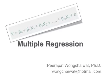
A linear regression model with more than one independent variable is called a multiple linear regression model .
We estimate the regression coefficients—called partial regression coefficients — b 0 , b 1 , b 2 ,… b k , then use the model: The partial regression coefficients represent the expected change in the dependent variable when the associated independent variable is increased by one unit while the values of all other independent variables are held constant .
The independent variables in the spreadsheet must be in contiguous columns. ◦ So, you may have to manually move the columns of data around before applying the tool. Key differences: Multiple R and R Square are called the multiple correlation coefficient and the coefficient of multiple determination , respectively, in the context of multiple regression. ANOVA tests for significance of the entire model. That is, it computes an F-statistic for testing the hypotheses:
ANOVA tests for significance of the entire model. That is, it computes an F-statistic for testing the hypotheses: The multiple linear regression output also provides information to test hypotheses about each of the individual regression coefficients. ◦ If we reject the null hypothesis that the slope associated with independent variable i is 0, then the independent variable i is significant and improves the ability of the model to better predict the dependent variable. If we cannot reject H0, then that independent variable is not significant and probably should not be included in the model.
Recommend
More recommend
Explore More Topics
Stay informed with curated content and fresh updates.
