Multiple Regression Peerapat Wongchaiwat, Ph.D. - PowerPoint PPT Presentation
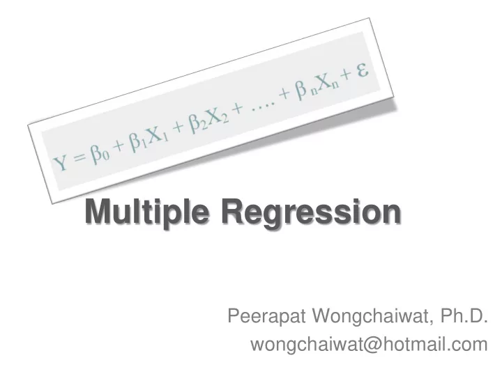
Multiple Regression Peerapat Wongchaiwat, Ph.D. wongchaiwat@hotmail.com The Multiple Regression Model Examine the linear relationship between 1 dependent (Y) & 2 or more independent variables (X i ) Multiple Regression Model with k
Multiple Regression Peerapat Wongchaiwat, Ph.D. wongchaiwat@hotmail.com
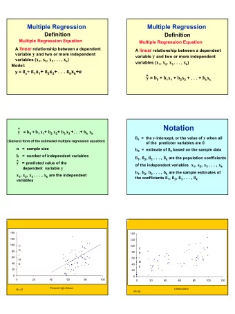
The Multiple Regression Model Examine the linear relationship between 1 dependent (Y) & 2 or more independent variables (X i ) Multiple Regression Model with k Independent Variables: Population slopes Random Error Y-intercept β β β β ε Y X X X 0 1 1 2 2 k k
Multiple Regression Equation The coefficients of the multiple regression model are estimated using sample data Multiple regression equation with k independent variables: Estimated Estimated Estimated slope coefficients (or predicted) intercept value of y ˆ y b b x b x b x i 0 1 1i 2 2i k k, i We will always use a computer to obtain the regression slope coefficients and other regression summary measures.
Sales Example Pie Price Advertising Multiple regression equation: Week Sales ($) ($100s) 1 350 5.50 3.3 2 460 7.50 3.3 Sales t = b 0 + b 1 (Price) t 3 350 8.00 3.0 + b 2 (Advertising) t + e t 4 430 8.00 4.5 5 350 6.80 3.0 6 380 7.50 4.0 7 430 4.50 3.0 8 470 6.40 3.7 9 450 7.00 3.5 10 490 5.00 4.0 11 340 7.20 3.5 12 300 7.90 3.2 13 440 5.90 4.0 14 450 5.00 3.5 15 300 7.00 2.7
Multiple Regression Output Regression Statistics Multiple R 0.72213 R Square 0.52148 Adjusted R Square 0.44172 Standard Error 47.46341 Sales 306.526 - 24.975(Pri ce) 74.131(Adv ertising) Observations 15 ANOVA df SS MS F Significance F Regression 2 29460.027 14730.013 6.53861 0.01201 Residual 12 27033.306 2252.776 Total 14 56493.333 Coefficients Standard Error t Stat P-value Lower 95% Upper 95% Intercept 306.52619 114.25389 2.68285 0.01993 57.58835 555.46404 Price -24.97509 10.83213 -2.30565 0.03979 -48.57626 -1.37392 Advertising 74.13096 25.96732 2.85478 0.01449 17.55303 130.70888
Adjusted 2 R • R 2 never decreases when a new X variable is added to the model, even if the new variable is not an important predictor variable – Hence, models with different number of explanatory variables cannot be compared by R 2 • What is the net effect of adding a new variable? – We lose a degree of freedom when a new X variable is added – Did the new X variable add enough explanatory power to offset the loss of one degree of freedom? * Adjusted R 2 penalizes excessive use of unimportant independent variables Adjusted R 2 is always smaller than R 2 ( except when R 2 =1)
F-Test for Overall Significance of the Model • Shows if there is a linear relationship between all of the X variables considered together and Y • Use F test statistic • Hypotheses: H 0 : β 1 = β 2 = … = β k = 0 (no linear relationship) H 1 : at least one β i ≠ 0 (at least one independent variable affects Y)
F-Test for Overall Significance (continued) Regression Statistics Multiple R 0.72213 MSR 14730.0 R Square 0.52148 F 6.5386 Adjusted R Square 0.44172 MSE 2252.8 Standard Error 47.46341 With 2 and 12 degrees of Observations 15 P-value for freedom the F-Test ANOVA df SS MS F Significance F Regression 2 29460.027 14730.013 6.53861 0.01201 Residual 12 27033.306 2252.776 Total 14 56493.333 Coefficients Standard Error t Stat P-value Lower 95% Upper 95% Intercept 306.52619 114.25389 2.68285 0.01993 57.58835 555.46404 Price -24.97509 10.83213 -2.30565 0.03979 -48.57626 -1.37392 Advertising 74.13096 25.96732 2.85478 0.01449 17.55303 130.70888
11-9 The ANOVA Table in Regression Source of Sum of Degrees of Variation Squares Freedom Mean Square F Ratio MSR Regression SSR (k) F SSR MSR MSE k SSE (n-(k+1)) Error SSE MSE =(n-k-1) ( 1 ) n k SST (n-1) Total SST MST ( 1 ) n SSE 2 SSR SSE ( ( 1 )) R 2 R n k (n - (k + 1)) = MSE R 2 = = 1 - F = 1 - 2 SST SST ( ) k ( 1 ) R MST SST (n - 1)
11-10 Tests of the Significance of Individual Regression Parameters Hypothesis tests about individual regression slope parameters: H 0 : b 1 = 0 (1) H 1 : b 1 0 H 0 : b 2 = 0 (2) H 1 : b 2 0 . . . H 0 : b k = 0 (k) H 1 : b k 0 0 b : Test statistic for test i t i ( n ( k 1 ) ( ) s b i
The Concept of Partial Regression Coefficients In multiple regression, the interpretation of slope coefficients requires special attention: ˆ y b b x b x i 0 1 1i 2 2i • Here, b 1 shows the relationship between X 1 and Y holding X 2 constant (i.e. controlling for the effect of X 2 ).
Purifying X 1 from X 2 (i.e. Removing the effect of X 2 on X 1 : Run a regression of X 2 on X 1 X 2i = 0 + 1 X 1i + v i v i = X 2i – ( 0 + 1 X 1i ) is X 2 purified from X 1 Then, run a regression of Y i on v i . Y i = 0 + 1 v i . 1 is the b 1 in the original multiple regression equation .
b 1 shows the relationship between X 1 purified from X 2 and Y. Whenever, a new explanatory variable is added into the regression equation or removed from from the equation, all b coefficients change. (unless, the covariance of the added or removed variable with all other variables is zero).
The Principle of Parsimony: Any insignificant explanatory variable should be removed out of the regression equation. The Principle of Generosity: Any significant variable must be included in the regression equation. Choosing the best model: Choose the model with the highest adjusted R 2 or F or the lowest AIC (Akaike Information Criterion) or SC (Schwarz Criterion). Apply the stepwise regression procedure.
Multiple Regression For example: A researcher may be interested in the relationship between Education and Income and Number of Children in a family. Independent Variables Dependent Variable Education Number of Children Family Income
Multiple Regression For example: Research Hypothesis: As education of respondents increases, the number of children in families will decline (negative relationship). Research Hypothesis: As family income of respondents increases, the number of children in families will decline (negative relationship). Independent Variables Dependent Variable Education Number of Children Family Income
Multiple Regression For example: Null Hypothesis: There is no relationship between education of respondents and the number of children in families. Null Hypothesis: There is no relationship between family income and the number of children in families. Independent Variables Dependent Variable Education Number of Children Family Income
Multiple Regression Bivariate regression is based on fitting a line as close as possible to the plotted coordinates of your data on a two-dimensional graph. Trivariate regression is based on fitting a plane as close as possible to the plotted coordinates of your data on a three-dimensional graph. Case: 1 2 3 4 5 6 7 8 9 10 11 12 13 14 15 16 17 18 19 20 21 22 23 24 25 Children (Y): 2 5 1 9 6 3 0 3 7 7 2 5 1 9 6 3 0 3 7 14 2 5 1 9 6 Education (X 1 ) 12 16 2012 9 18 16 14 9 12 12 10 20 11 9 18 16 14 9 8 12 10 20 11 9 Income 1=$10K (X 2 ): 3 4 9 5 4 12 10 1 4 3 10 4 9 4 4 12 10 6 4 1 10 3 9 2 4
Multiple Regression Y Plotted coordinates (1 – 10) for Education, Income and Number of Children 0 X 2 X 1 Case: 1 2 3 4 5 6 7 8 9 10 11 12 13 14 15 16 17 18 19 20 21 22 23 24 25 Children (Y): 2 5 1 9 6 3 0 3 7 7 2 5 1 9 6 3 0 3 7 14 2 5 1 9 6 Education (X 1 ) 12 16 2012 9 18 16 14 9 12 12 10 20 11 9 18 16 14 9 8 12 10 20 11 9 Income 1=$10K (X 2 ): 3 4 9 5 4 12 10 1 4 3 10 4 9 4 4 12 10 6 4 1 10 3 9 2 4
Multiple Regression Y What multiple regression does is fit a plane to these coordinates. 0 X 2 X 1 Case: 1 2 3 4 5 6 7 8 9 10 Children (Y): 2 5 1 9 6 3 0 3 7 7 Education (X 1 ) 12 16 2012 9 18 16 14 9 12 Income 1=$10K (X 2 ): 3 4 9 5 4 12 10 1 4 3
Multiple Regression • Mathematically, that plane is: Y = a + b 1 X 1 + b 2 X 2 a = y-intercept, where X ’ s equal zero b=coefficient or slope for each variable For our problem, SPSS says the equation is: Y = 11.8 - .36X 1 - .40X 2 Expected # of Children = 11.8 - .36*Educ - .40*Income
Multiple Regression • Let ’ s take a moment to reflect… Why do I write the equation: Y = a + b 1 X 1 + b 2 X 2 Whereas KBM often write: Y i = a + b 1 X 1 i + b 2 X 2 i + e i One is the equation for a prediction, the other is the value of a data point for a person.
Recommend
More recommend
Explore More Topics
Stay informed with curated content and fresh updates.
