STAT 213 Interactions in Multiple Regression Colin Reimer Dawson - PowerPoint PPT Presentation

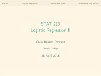
Outline Refresher: The Multiple Regression Model STAT 213 Interactions in Multiple Regression Colin Reimer Dawson Oberlin College 29 March 2016

Outline Refresher: The Multiple Regression Model Outline Refresher: The Multiple Regression Model Defining the Model R 2 and Parsimony CIs and PIs for MLR

Outline Refresher: The Multiple Regression Model Reading Quiz An environmental expert is interested in modeling the concentration of various chemicals in well water over time. Identify the regression model that would be used to predict the amount of lead ( Lead ) in a well based on Year , with two different lines depending on whether or not the well has been cleaned ( Iclean ).

Outline Refresher: The Multiple Regression Model For Thursday • Read: 4.4, 7.5 • Write up (as a lab): 3.20, 3.30 • Answer: 4.12, 7.30

Outline Refresher: The Multiple Regression Model Outline Refresher: The Multiple Regression Model Defining the Model R 2 and Parsimony CIs and PIs for MLR

Outline Refresher: The Multiple Regression Model Outline Refresher: The Multiple Regression Model Defining the Model R 2 and Parsimony CIs and PIs for MLR

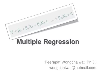
Outline Refresher: The Multiple Regression Model The Multiple Regression Model DATA = PATTERN + IDIOSYNCRACIES The Multiple Regression Population Model Y = f ( X 1 , . . . , X K ) + ε Y = β 0 + β 1 X 1 + · · · + β k X k + ε One β j for each predictor X j

Outline Refresher: The Multiple Regression Model The Four-Step Process: Multiple Regression 1. CHOOSE a form of the model • Select predictors • Choose any transformations of predictors 2. FIT: Estimate • coefficients: ˆ β 1 , ˆ β 1 , . . . , ˆ β k • residual variance ˆ σ 2 ε 3. ASSESS the fit • Examine residuals • Test individual predictors ( t -tests) • Test overall fit (ANOVA, R 2 ) 4. USE the model • Make predictions • Construct CIs and PIs

Outline Refresher: The Multiple Regression Model Checking Conditions Same conditions as always apply: 1. Linearity (mean of Y is given by some linear model) 2. Independence (residuals are not correlated) 3. Homoskedasticity (same variance at all combinations of X ) 4. Normality (residuals normally distributed)

Outline Refresher: The Multiple Regression Model Testing Individual Predictors ( t -tests) library(Stat2Data); data("Pulse") PulseWithBMI <- mutate( Pulse, BMI = Wgt / Hgt^2 * 703, InvActive = 1 / Active, InvRest = 1 / Rest, Male = 1 - Gender) active.model <- lm(InvActive ~ InvRest + Hgt + BMI, data = PulseWithBMI)

Outline Refresher: The Multiple Regression Model summary(active.model) Call: lm(formula = InvActive ~ InvRest + Hgt + BMI, data = PulseWithBMI) Residuals: Min 1Q Median 3Q Max -0.0053245 -0.0010301 0.0000241 0.0011322 0.0052298 Coefficients: Estimate Std. Error t value Pr(>|t|) (Intercept) 3.333e-04 2.187e-03 0.152 0.8790 InvRest 6.506e-01 5.547e-02 11.728 <2e-16 *** Hgt 5.125e-05 3.376e-05 1.518 0.1304 BMI -9.052e-05 3.875e-05 -2.336 0.0204 * --- Signif. codes: 0 '***' 0.001 '**' 0.01 '*' 0.05 '.' 0.1 ' ' 1 Residual standard error: 0.001787 on 228 degrees of freedom Multiple R-squared: 0.4026,Adjusted R-squared: 0.3947 F-statistic: 51.21 on 3 and 228 DF, p-value: < 2.2e-16

Outline Refresher: The Multiple Regression Model Controls In the context of a multiple regression model, the t -test for a predictor tests for a linear association after controlling for the other predictors .

Outline Refresher: The Multiple Regression Model Testing the Overall Model H 0 : β 1 = β 2 = · · · = β k = 0 H 1 : Some β j � = 0 i =1 (ˆ Y i − ¯ � n Y ) 2 /k F = MS Model = � n i =1 ( Y i − ˆ MS Error Y i ) / ( n − k − 1) 0.8 density 0.6 0.4 0.2 1 2 3 4 5

Outline Refresher: The Multiple Regression Model Adjusted R 2 • R 2 can only go up as we add predictors, because at worst, we can choose β k +1 = β k ′ = 0 and get the same SSE. Usually we can pick coefficients to do somewhat better. • Would like to “penalize” unnecessary predictors.

Outline Refresher: The Multiple Regression Model Adjusted R 2 adj = 1 − SS Error / ( n − k − 1) R 2 SS Total / ( n − 1) σ 2 = 1 − ˆ ε s 2 Y 1 − R 2 1 − R 2 adj = d f Error /d f Total

Outline Refresher: The Multiple Regression Model Outline Refresher: The Multiple Regression Model Defining the Model R 2 and Parsimony CIs and PIs for MLR

Outline Refresher: The Multiple Regression Model What happens to R 2 as we add predictors? Worksheet

Outline Refresher: The Multiple Regression Model What Makes a Good Model? Fit Validity High R 2 Strong evidence for predictors Small SSE Simple (Parsimonious) Large F Generalizes outside sample

Outline Refresher: The Multiple Regression Model Why Does Parsimony Matter? Don’t we just care about good predictions? Not exclusively... • We also use models to understand the world (harder with more complexity) And even so... • We really care about making predictions for data we haven’t seen yet .

Outline Refresher: The Multiple Regression Model Outline Refresher: The Multiple Regression Model Defining the Model R 2 and Parsimony CIs and PIs for MLR

Outline Refresher: The Multiple Regression Model CIs and PIs Confidence and Prediction Intervals have same interpretation as in the single predictor case: • C % CI: Procedure to produce an interval at a particular ( X 1 , . . . , X k ) that will contain the true ˆ Y for C % of data sets. • C % PI: Procedure to produce an interval at a particular ( X 1 , . . . , X k ) that will contain the true Y for C % of “datasets plus a case”.