Multiple Regression and Logistic Regression II Dajiang Liu @PHS - PowerPoint PPT Presentation

Multiple Regression and Logistic Regression II Dajiang Liu @PHS 525 Apr-19-2016

Materials from Last Time • Multiple regression model: • Include multiple predictors in the model � � = � � + � � � �� + � � � �� + ⋯ + � � • How to interpret the parameter estimate: • � � represent the change in � � per unit of change in � �� given � �,� , … , � �,��� , � �,��� unchanged. • Measures for model fitting • � � � • � ���

Two Types of P-values • P-values for the assessment of model fitting • � � : � � = ⋯ = � � = 0 • � � : � � ≠ 0 or � � ≠ 0 or … � � ≠ 0 • P-values for testing the statistical significance for each predictor • � � : � � = 0 • � � : � � ≠ 0

Questions of Interest • Not all predictors are useful • Including “not useful” predictors in the model will reduce the accuracy of predictors • Full model is the model that contains all predictors • Question: Determine useful predictors from the full model

Approach I • Fit the full model that contains the full set of predictors • Determine which predictors are important by looking at • P-values for testing � � : � � = 0 • Predictor � is important if p-values are significant for testing � �

Mario_Kart Example Revisited • Fit the full model including all predictors • Cond • Wheels • Duration • Stock_photo • Which variables are important? Why?

Approach II • Use of goodness of fit � � • Larger values of � � (or � ��� � ) indicate the model is better • Usually more preferred than the approach for examining each p- values for each predictor

Two Model Selection Strategies I – � Backward Elimination Using � ��� Backward Elimination Backward Elimination Backward Elimination as a Criterion • Backward Elimination • Step 1: Fit the full model • Step 2: Remove the predictor with the least significant p-values � • Step 3: Compare new model and old model based upon � ��� � • Step 4: Repeat step 2 and 3 until the values for � ��� do not change “much”

Two Model Selection Strategies II – Forward Selection Forward Selection Forward Selection Forward Selection • Forward selection • Step 1: Fit the null model with no predictors • Step 2: Examine each predictor, and add the predictor with the most significant p-values � • Step 3: Compare new model and old model based upon � ��� � • Step 4: Add the predictor if there � ��� change significantly. If the values for � � ��� do not change much with all predictors, stop

Model Selection Using Akaike Information Criterion • With more predictors, the fitting will always be better • Even when the predictors are not good • You need to penalize the number of parameter models � • Instead of directing using � ��� • AIC is sometimes used, which equals to ��� = 2 − 2log (&)

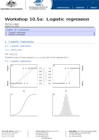
Logistic regression – Motivation • The response variable may not be normally distributed • E.g. the response is a categorical variable • When response variables are binary, a new method “generalized linear model” is used • Two step modeling: • Step 1: model the response as a random variable, following a distribution (say binomial or Poisson) • Step 2: model the parameters of the distribution as function of the predictors

Email Data Revisited

Modeling the Probability for the Response • When the response is two-level categorical variable (e.g. Yes or No), logistic regression model can be used to model the response • We denote � � as the response variable. � � takes two values 0 and 1. • We denote the probability of � � having value of 1 as ( � = Pr � � = 1 . • The probability for Pr � � = 0 = 1 − ( � .

Model the Event Probability as Functions of the Predictors • A GLM-based multiple regression model usually takes the form ,-./012-3 ( � = � � + � � � � + ⋯ + � 4 � 4 • The transformation can be the logit function ( � logit ( � = log 1 − ( � • GLMs using logit as link function is called logistic regression ( � log = � � + � � � � + ⋯ + � 4 � 4 1 − ( �

What does Logistic Link Function Look Like? The logit for a probability has range from (-Inf,Inf) 6 4 2 logit.p 0 -2 -4 -6 0.0 0.2 0.4 0.6 0.8 1.0 p

Interpret the Coefficients I • The parameters estimated in logistic regression models can be used to estimate the probability of the response variables: • Example: in the Email dataset, regressing variable 7(.3 on the variable ,2_39:,;(:< , we obtain ( � log = − 2.12 − 1.81 × ,2_39:,;(:< 1 − ( � • Question: What is the probability of a given email being a spam?

Interpreting the Coefficients II • Using simple linear regression model, we have exp −2.12 − 1.81 × ,2_39:,;(:< (̂ � = 1 + exp −2.12 − 1.81 × ,2_39:,;(:< • What is the predicted probability for an email being spam if it is sent to multiple users?

Interpreting the Coefficients III • How to interpret the parameter estimates from logistic regression model: • The coefficient estimates represent log odds ratio : What is an odds: D � = Pr � � = 1 � � = 1 / Pr � � = 0 � � = 1 D � = Pr � � = 1 � � = 0 / Pr � � = 0 � � = 0 What is an odds ratio: D� = D � /D �

Odds ratio F G • Using the simplest model log ��F G = � � + � � � � • D � = Pr � � = 1 � � = 1 /Pr (� � = 0 � � = 1 = exp (� � + � � ) • D � = Pr � � = 1 � � = 0 /Pr (� � = 0 � � = 0 = exp (� � ) H I • D� = H J = exp � � • log D� = � �

A Tabular View of Odds Ratio • The odds ratio can be calculated by the quotient of the product of diagonal element over the product of the off-diagonal element: K = L K = M � = 0 Pr(� = 0|� = 0) Pr(� = 1|� = 0) � = 1 Pr(� = 0|� = 1) Pr(� = 1|� = 1)

Practical Exercise: • Email dataset revisited: • Can you repeat the analyses regressing SPAM over to_multiple? data=read.table('email.txt',header=T,sep='\t'); summary(data) names(data) summary(glm(spam~to_multiple,data=data,family='binomial'))

Any Other Variables Important to SPAM classification? • Perform multiple logistic regression models • Similar to multiple linear regression, multiple logistic regression models can be performed to incorporate multiple predictors ( � log = � � + � � � �� + � � � �� + � O � �O 1 − ( � • How to interpret the parameters?

Email Data: Multiple Predictors • Include addition predictors into the model summary(glm(spam ~ to_multiple + cc + image + attach + winner + dollar,family='binomial',data=data)) Call: glm(formula = spam ~ to_multiple + cc + image + attach + winner + dollar, family = "binomial", data = data) Deviance Residuals: Min 1Q Median 3Q Max -2.4908 -0.4744 -0.4744 -0.2020 3.5959 Coefficients: Estimate Std. Error z value Pr(>|z|) (Intercept) -2.12767 0.06176 -34.450 < 2e-16 *** to_multiple -2.01934 0.30788 -6.559 5.42e-11 *** cc 0.01770 0.02102 0.842 0.399659 image -4.98117 2.11866 -2.351 0.018718 * attach 0.72125 0.11335 6.363 1.98e-10 *** winneryes 1.88412 0.29818 6.319 2.64e-10 *** dollar -0.07626 0.02018 -3.779 0.000157 *** --- Signif. codes: 0 ‘***’ 0.001 ‘**’ 0.01 ‘*’ 0.05 ‘.’ 0.1 ‘ ’ 1 (Dispersion parameter for binomial family taken to be 1) Null deviance: 2437.2 on 3920 degrees of freedom Residual deviance: 2271.5 on 3914 degrees of freedom AIC: 2285.5 Number of Fisher Scoring iterations: 9