Notation ^ y = b 0 + b 1 x 1 + b 2 x 2 + b 3 x 3 +. . .+ b k x k 0 - PDF document

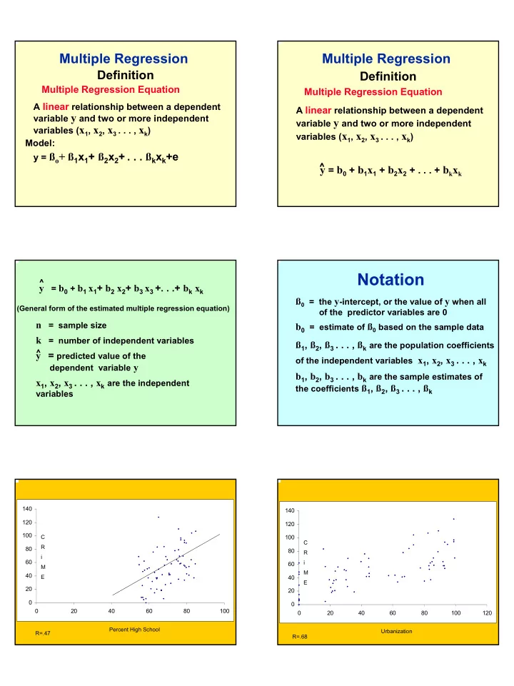
Multiple Regression Multiple Regression Definition Definition Multiple Regression Equation Multiple Regression Equation A linear relationship between a dependent A linear relationship between a dependent variable y and two or more independent variable y and two or more independent variables ( x 1 , x 2 , x 3 . . . , x k ) variables ( x 1 , x 2 , x 3 . . . , x k ) Model: y = ß o + ß 1 x 1 + ß 2 x 2 + . . . ß k x k +e ^ y = b 0 + b 1 x 1 + b 2 x 2 + . . . + b k x k Notation ^ y = b 0 + b 1 x 1 + b 2 x 2 + b 3 x 3 +. . .+ b k x k ß 0 = the y -intercept, or the value of y when all (General form of the estimated multiple regression equation) of the predictor variables are 0 n = sample size b 0 = estimate of ß 0 based on the sample data k = number of independent variables ß 1 , ß 2 , ß 3 . . . , ß k are the population coefficients ^ y = predicted value of the of the independent variables x 1 , x 2 , x 3 . . . , x k dependent variable y b 1 , b 2 , b 3 . . . , b k are the sample estimates of x 1 , x 2 , x 3 . . . , x k are the independent the coefficients ß 1 , ß 2 , ß 3 . . . , ß k variables 140 140 120 120 100 C 100 C R 80 80 R i 60 i 60 M M 40 E 40 E 20 20 0 0 0 20 40 60 80 100 0 20 40 60 80 100 120 Percent High School Urbanization R=.47 R=.68

Analysis of Variance Sum of Mean Source DF Squares Square F Value Pr > F Model 2 24732 12366 28.54 <.0001 Error 64 27730 433.28847 Corrected Total 66 52462 Overall Regression Analysis: A Test of the Multiple R Root MSE 20.81558 R-Square 0.4714 Parameter Estimates (R=.686) Parameter Standard Dependent Mean 52.40299 Adj R-Sq 0.4549 Variable DF Estimate Error t Value Pr > |t| Intercept 1 59.11807 28.36531 2.08 0.0411 Coeff Var 39.72213 hs 1 -0.58338 0.47246 -1.23 0.2214 Urb 1 0.68250 0.12321 5.54 <.0001 Notice that the slope of hs is negative Pearson Correlation Coefficients, N = 67 Parameter Estimates Prob > |r| under H0: Rho=0 crate incom hs Urb crate 1.00000 0.43375 0.46691 0.67737 Parameter Standard 0.0002 <.0001 <.0001 Variable DF Estimate Error t Value Pr > |t| Intercept 1 -50.85690 24.45065 -2.08 0.0415 incom 0.43375 1.00000 0.79262 0.73070 0.0002 <.0001 <.0001 hs 1 1.48598 0.34908 4.26 <.0001 hs 0.46691 0.79262 1.00000 0.79072 <.0001 <.0001 <.0001 Urb 0.67737 0.73070 0.79072 1.00000 When hs is by itself the slope is positive <.0001 <.0001 <.0001

Adjusted R 2 Multiple Regression SAS Setup Definitions • proc corr ; run ; � Multiple coefficient of determination • proc reg ; model crate= hs Urb; a measure of how well the multiple • plot crate*hs; run ; regression equation fits the sample data • proc reg ; model crate= hs; run ; � Adjusted coefficient of determination the multiple coefficient of determination R 2 modified to account for the number of variables and the sample size Adjusted R Adjusted R 2 2 2 = 1 - ( n - 1) 2 ) ( 1 - R Adjusted R [ n - ( k + 1) ] Including the Three Variables Adjusted R 2 Analysis of Variance 2 = 1 - ( n - 1) 2 ) Adjusted R ( 1 - R Sum of Mean [ n - ( k + 1) ] Source Squares Square F Value Pr > F DF Model 3 24804 8268.16424 18.83 <.0001 Error 63 27658 439.00995 where n = sample size k = number of independent ( x ) variables Corrected Total 66 52462

Overall Test Tests of Hypotheses Root MSE 20.95256 R-Square 0.4728 • Overall test: Null: All of the population regression weights are zero. Dependent Mean 52.40299 Adj R-Sq 0.4477 Alternative: Not all are zero Coeff Var 39.98353 Parameter Estimates The overall F Test Parameter Standard Variable DF Estimate Error t Value Pr > |t| Intercept 1 59.71473 28.58953 2.09 0.0408 2 R / k = F − − k , n k 1 incom 1 -0.38309 0.94053 -0.41 0.6852 2 − − − ( 1 R ) /( n k 1 ) hs 1 -0.46729 0.55443 -0.84 0.4025 Urb 1 0.69715 0.12913 5.40 <.0001 Individual Tests F Test for Restricted Models • Test for b 1 : Y = b o + b 1 x 1 + b 2 x 2 + b 3 x 3 + e Y = b o + b 2 x 2 + b 3 x 3 + e 2 2 − − ( R R ) /( k g ) • Test for b 2 : f r = F − − − Y = b o + b 1 x 1 + b 2 x 2 + b 3 x 3 + e k g , n k 1 2 − − − ( 1 R ) /( n k 1 ) Y = b o + b 1 x 1 + b 3 x 3 + e f • Test for b 3 : Y = b o + b 1 x 1 + b 2 x 2 + b 3 x 3 + e Y = b o + b 1 x 1 + b 2 x 2 + e

More on SAS Standardized Regression Weights • Model options:   S x   * Model y = x1 x2 / R partial p stb; = i b b i i   R– residual analysis S   y Partial– partial regression scatter plot P– predicted values Stb– standardized regression weights Generally, the standardized regression weights fall between 1 and –1. However, they can larger than one (or less than –1). Parameter Estimates Obtaining the Standardized Parameter Standard Standardized Regression Weights Variable DF Estimate Error t Value Pr > |t| Estimate • Model Statement Intercept 1 59.71473 28.58953 2.09 0.0408 0 – Model crate = incom hs urb /stb; incom 1 -0.38309 0.94053 -0.41 0.6852 -0.06363 hs 1 -0.46729 0.55443 -0.84 0.4025 -0.14683 Urb 1 0.69715 0.12913 5.40 <.0001 0.83996 „ƒˆƒƒƒƒƒˆƒƒƒƒƒˆƒƒƒƒƒˆƒƒƒƒƒˆƒƒƒƒƒˆƒƒƒƒƒˆƒƒƒƒƒˆƒƒƒƒƒˆƒƒƒƒƒˆƒƒƒƒƒˆƒƒƒƒƒˆƒƒƒƒƒˆƒƒƒƒƒˆƒƒƒƒƒˆƒƒ† crate ‚ ‚ Partial Regression Plots ‚ ‚ ‚ ‚ ‚ ‚ ‚ ‚ 60 ˆ ˆ ‚ ‚ ‚ ‚ ‚ 1 ‚ ‚ 1 ‚ ‚ ‚ 40 ˆ 1 ˆ • Plot of two residuals ‚ 1 1 ‚ ‚ 1 ‚ ‚ ‚ ‚ 1 1 1 ‚ ‚ 1 ‚ • The regression line in this plot corresponds 20 ˆ 1 1 1 ˆ ‚ 1 1 1 11 1 1 ‚ Crate-b 1 (inc)-b 2 (urb) ‚ 1 1 1 ‚ ‚ 1 1 1 ‚ to the regression weight in the overall ‚ ‚ ‚ 1 ‚ 0 ˆ 1 1 ˆ ‚ 1 1 1 ‚ ‚ 1 1 1 1 ‚ model. ‚ 1 1 2 ‚ ‚ 1 1 1 1 1 11 1 1 ‚ ‚ 1 1 1 1 1 1 1 ‚ -20 ˆ 2 1 ˆ • Model Statement ‚ 2 1 1 ‚ ‚ 1 ‚ ‚ ‚ ‚ 1 1 ‚ ‚ 1 ‚ / partial -40 ˆ ˆ ‚ ‚ ‚ ‚ ‚ ‚ ‚ ‚ ‚ ‚ ŠƒˆƒƒƒƒƒˆƒƒƒƒƒˆƒƒƒƒƒˆƒƒƒƒƒˆƒƒƒƒƒˆƒƒƒƒƒˆƒƒƒƒƒˆƒƒƒƒƒˆƒƒƒƒƒˆƒƒƒƒƒˆƒƒƒƒƒˆƒƒƒƒƒˆƒƒƒƒƒˆƒƒƒƒƒˆƒƒŒ -14 -12 -10 -8 -6 -4 -2 0 2 4 6 8 10 12 14 hs Hs-b 1 (inc)-b 2 (urb)

„ƒˆƒƒƒƒƒƒˆƒƒƒƒƒƒˆƒƒƒƒƒƒˆƒƒƒƒƒƒˆƒƒƒƒƒƒˆƒƒƒƒƒƒˆƒƒƒƒƒƒˆƒƒƒƒƒƒˆƒƒƒƒƒƒˆƒƒƒƒƒƒˆƒƒƒƒƒƒˆƒƒƒƒƒƒˆƒƒ† crate ‚ ‚ ‚ ‚ Interaction of two Variables ‚ ‚ 80 ˆ ˆ ‚ 1 ‚ ‚ ‚ ‚ ‚ ‚ ‚ 60 ˆ ˆ ‚ ‚ ‚ ‚ ‚ 1 ‚ ‚ ‚ • Just as in ANOVA we can have interaction effects 40 ˆ 1 1 ˆ ‚ 1 1 1 ‚ ‚ 11 ‚ in a multiple regression analysis. ‚ 1 1 ‚ ‚ 1 1 ‚ Crate-b 1 (inc)-b 2 (hs) 20 ˆ 1 1 1 1 1 1 ˆ ‚ 1 ‚ • For quantitative variables, interaction is present ‚ 1 1 ‚ ‚ 1 1 1 1 ‚ ‚ 1 1 1 1 1 ‚ 0 ˆ ˆ when the relationship between the explanatory ‚ 1 1 1 1 1 ‚ ‚ 1 1 1 1 11 ‚ ‚ 1 1 ‚ variable and the response changes as the levels of ‚ 1 1 1 1 1 ‚ -20 ˆ 1 1 ˆ ‚ 1 1 1 ‚ another variable changes. ‚ 1 1 12 1 1 1 ‚ ‚ 1 1 ‚ ‚ 1 1 ‚ -40 ˆ ˆ • Consider crime rate as a function of hs and urb. If ‚ 1 ‚ ‚ ‚ ‚ ‚ the relationship (slope) between crime rate and urb ‚ ‚ -60 ˆ ˆ ‚ ‚ changes as hs changes, we have an interaction ‚ ‚ ŠƒˆƒƒƒƒƒƒˆƒƒƒƒƒƒˆƒƒƒƒƒƒˆƒƒƒƒƒƒˆƒƒƒƒƒƒˆƒƒƒƒƒƒˆƒƒƒƒƒƒˆƒƒƒƒƒƒˆƒƒƒƒƒƒˆƒƒƒƒƒƒˆƒƒƒƒƒƒˆƒƒƒƒƒƒˆƒƒŒ -60 -50 -40 -30 -20 -10 0 10 20 30 40 50 60 between urb and hs. Urb Urb-b 1 (inc)-b 2 (hs) Testing for an Interaction Effect SAS Setup for Interaction • We test for interaction effect by comparing • Create a the product variable in the data a model with interaction to a model without statement: interaction: – Data new; input y x z; xz=x*z; cards; Y = β o + β 1 x 1 + β 2 x 2 + β 3 (x 1 *x 2 ) + e Y = β o + β 1 x 1 + β 2 x 2 + e – Model y = x z xz; Parameter Estimates Root MSE 20.82583 R-Square 0.4792 Parameter Standard Variable DF Estimate Error t Value Pr > |t| Dependent Mean 52.40299 Adj R-Sq 0.4544 Intercept 1 19.31754 49.95871 0.39 0.7003 hs 1 0.03396 0.79381 0.04 0.9660 Coeff Var 39.74168 Urb 1 1.51431 0.86809 1.74 0.0860 hsurb 1 -0.01205 0.01245 -0.97 0.3367 Model crate= hs urb hs*urb (Looking for an interaction) Testing the Interaction