Simple Linear Regression Recall: A regression model describes how a - PowerPoint PPT Presentation

ST 430/514 Introduction to Regression Analysis/Statistics for Management and the Social Sciences II Simple Linear Regression Recall: A regression model describes how a dependent variable (or response ) Y is affected, on average, by one or more independent variables (or factors , or covariates ) x 1 , x 2 , . . . , x k . 1 / 20 Simple Linear Regression Introduction

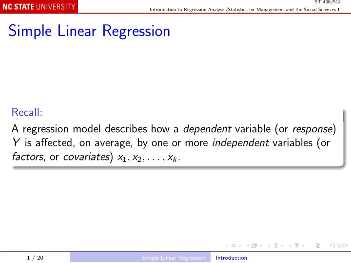
ST 430/514 Introduction to Regression Analysis/Statistics for Management and the Social Sciences II The Straight-Line Probabilistic Model Simplest case of a regression model: One independent variable, k = 1, x 1 ≡ x ; Linear dependence; Model equation: E ( Y ) = β 0 + β 1 x , or equivalently Y = β 0 + β 1 x + ǫ. 2 / 20 Simple Linear Regression The Straight-Line Probabilistic Model

ST 430/514 Introduction to Regression Analysis/Statistics for Management and the Social Sciences II Interpreting the parameters: β 0 is the intercept (so called because it is where the graph of y = β 0 + β 1 x meets the y -axis x = 0); β 1 is the slope ; that is, the change in E ( y ) as x is changed to x + 1. Note: if β 1 = 0, x has no effect on y ; that will often be an interesting hypothesis to test. 3 / 20 Simple Linear Regression The Straight-Line Probabilistic Model

ST 430/514 Introduction to Regression Analysis/Statistics for Management and the Social Sciences II Advertising and Sales example x = monthly advertising expenditure, in hundreds of dollars; y = monthly sales revenue, in thousands of dollars; β 0 = expected revenue with no advertising; β 1 = expected revenue increase per $100 increase in advertising, in thousands of dollars. Sample data for five months: Advertising 1 2 3 4 5 Revenue 1 1 2 2 4 4 / 20 Simple Linear Regression The Straight-Line Probabilistic Model

ST 430/514 Introduction to Regression Analysis/Statistics for Management and the Social Sciences II What do these data tell about β 0 and β 1 ? Advertising and revenue scatterplot 4 ● 3 ● ● y 2 1 ● ● 0 0 1 2 3 4 5 x 5 / 20 Simple Linear Regression The Straight-Line Probabilistic Model

ST 430/514 Introduction to Regression Analysis/Statistics for Management and the Social Sciences II We could try various values of β 0 and β 1 . For given values of β 0 and β 1 , we get predictions p i = β 0 + β 1 x i , i = 1 , 2 , 3 , 4 , 5 . The difference betweem the observed value y i and the prediction p i is the residual r i = y i − p i , i = 1 , 2 , 3 , 4 , 5 . A good choice of β 0 and β 1 gives accurate predictions, and generally small residuals. 6 / 20 Simple Linear Regression The Straight-Line Probabilistic Model

ST 430/514 Introduction to Regression Analysis/Statistics for Management and the Social Sciences II One candidate line ( β 0 = − 0 . 1 , β 1 = 0 . 7): Advertising and revenue with candidate line 4 ● 3 2 ● ● y 1 ● ● 0 0 1 2 3 4 5 x 7 / 20 Simple Linear Regression The Straight-Line Probabilistic Model

ST 430/514 Introduction to Regression Analysis/Statistics for Management and the Social Sciences II Fitting the Model How to measure the overall size of the residuals? Most common measure (but not the only possibility): sum of squares of residuals � � r 2 ( y i − p i ) 2 i = � { y i − ( β 0 + β 1 x i ) } 2 = = S ( β 0 , β 1 ) . The least squares line is the one with the smallest sum of squares. Note: the least squares line has the property that � r i = 0; Definition 3.1 (page 95) does not need to impose that as a constraint. 8 / 20 Simple Linear Regression Fitting the Model

ST 430/514 Introduction to Regression Analysis/Statistics for Management and the Social Sciences II The least squares estimates of β 0 and β 1 are the coefficients of the least squares line. Some algebra shows that the least squares estimates are � x i y i − n ¯ � ( x i − ¯ x )( y i − ¯ y ) x ¯ y ˆ β 1 = = � x 2 � ( x i − ¯ x ) 2 i − n ¯ x 2 and ˆ y − ˆ β 0 = ¯ β 1 ¯ x . With a little luck, you will never need to use these formulæ. 9 / 20 Simple Linear Regression Fitting the Model

ST 430/514 Introduction to Regression Analysis/Statistics for Management and the Social Sciences II Other criteria Why square the residuals? We could use least absolute deviations estimates, minimizing � S 1 ( β 0 , β 1 ) = | y i − ( β 0 + β 1 x i ) | . Convenience: we have equations for the least squares estimates, but to find the least absolute deviations estimates we have to solve a linear programming problem. Optimality: least squares estimates are BLUE if the errors ǫ are uncorrelated with constant variance, and MVUE if additionally ǫ is normal. 10 / 20 Simple Linear Regression Fitting the Model

ST 430/514 Introduction to Regression Analysis/Statistics for Management and the Social Sciences II Model Assumptions The least squares line gives point estimates of β 0 and β 1 . These estimates are always unbiased. To use the other forms of statistical inference: interval estimates, such as confidence intervals; hypothesis tests; we need some assumptions about the random errors ǫ . 11 / 20 Simple Linear Regression Model Assumptions

ST 430/514 Introduction to Regression Analysis/Statistics for Management and the Social Sciences II Zero mean : E ( ǫ i ) = 0; as noted earlier, this is not really an 1 assumption, but a consequence of the definition ǫ = Y − E ( Y ) . Constant variance : V ( ǫ i ) = σ 2 ; this is a nontrivial assumption, 2 often violated in practice. Normality : ǫ i ∼ N (0 , σ 2 ); this is also a nontrivial assumption, 3 always violated in practice, but sometimes a useful approximation. Independence : ǫ i and ǫ j are statistically independent ; another 4 nontrivial assumption, often true in practice, but typically violated with time series and spatial data. 12 / 20 Simple Linear Regression Model Assumptions

ST 430/514 Introduction to Regression Analysis/Statistics for Management and the Social Sciences II Notes: Assumptions 2 and 4 are the conditions under which least squares estimates are BLUE (Best Linear Unbiased Estimators); Assumptions 2, 3, and 4 are the conditions under which least squares estimates are MVUE (Minimum Variance Unbiased Estimators). 13 / 20 Simple Linear Regression Model Assumptions

ST 430/514 Introduction to Regression Analysis/Statistics for Management and the Social Sciences II Estimating σ 2 Recall that σ 2 is the variance of ǫ i , which we have assumed to be the same for all i . That is, σ 2 = V ( ǫ i ) = V [ Y i − E ( Y i )] = V [ Y i − ( β 0 + β 1 x i )] , i = 1 , 2 , . . . , n . We observe Y i = y i and x i ; if we knew β 0 and β 1 , we would estimate σ 2 by 1 { y i − ( β 0 + β 1 x i ) } 2 = 1 � nS ( β 0 , β 1 ) . n An Estimator of σ 2 14 / 20 Simple Linear Regression

ST 430/514 Introduction to Regression Analysis/Statistics for Management and the Social Sciences II We do not know β 0 and β 1 , but we have least squares estimates ˆ β 0 and ˆ β 1 . � � β 0 , ˆ ˆ So we could use S as an approximation to S ( β 0 , β 1 ). β 1 � � β 0 , ˆ ˆ But we know that S β 1 < S ( β 0 , β 1 ), so 1 � � β 0 , ˆ ˆ nS β 1 would be a biased estimate of σ 2 . An Estimator of σ 2 15 / 20 Simple Linear Regression

ST 430/514 Introduction to Regression Analysis/Statistics for Management and the Social Sciences II We can show that, under Assumptions 2 and 4, � � �� β 0 , ˆ ˆ = ( n − 2) σ 2 . E S β 1 So 1 1 s 2 = � � β 0 , ˆ ˆ � y i ) 2 , n − 2 S β 1 = ( y i − ˆ n − 2 y i = ˆ β 0 + ˆ β 1 x i , is an unbiased estimate of σ 2 . where ˆ This is sometimes written s 2 = Mean Square for Error = MS E degrees of freedom for Error = SS E Sum of Squares for Error = . df E An Estimator of σ 2 16 / 20 Simple Linear Regression

ST 430/514 Introduction to Regression Analysis/Statistics for Management and the Social Sciences II Inferences about the line We are often interested in the question of whether x has any effect on E ( Y ). Since E ( Y ) = β 0 + β 1 x , the independent variable x has some effect whenever β 1 � = 0. So we need to test the null hypothesis H 0 : β 1 = 0. 17 / 20 Simple Linear Regression Making Inferences About the Slope β 1

ST 430/514 Introduction to Regression Analysis/Statistics for Management and the Social Sciences II We also need to construct a confidence interval for β 1 , to indicate how precisely we know its value. For both purposes, we need the standard error : σ β 1 = √ SS xx σ ˆ , where � x ) 2 . SS xx = ( x i − ¯ As always, since σ is unknown, we replace it by its estimate s , to get the estimated standard error s ˆ β 1 = √ SS xx σ ˆ . 18 / 20 Simple Linear Regression Making Inferences About the Slope β 1

ST 430/514 Introduction to Regression Analysis/Statistics for Management and the Social Sciences II A confidence interval for β 1 is ˆ β 1 ± t α/ 2 , n − 2 × ˆ σ ˆ β 1 . Note that we use the t -distribution with n − 2 degrees of freedom, because that is the degrees of freedom associated with s 2 . To test H 0 : β 1 = 0, we use the test statistic ˆ β 1 t = , σ ˆ ˆ β 1 and reject H 0 at the significance level α if | t | > t α/ 2 , n − 2 . 19 / 20 Simple Linear Regression Making Inferences About the Slope β 1