Regression: Simple and Linear Introduction to Machine Learning - PowerPoint PPT Presentation
INTRODUCTION TO MACHINE LEARNING Regression: Simple and Linear Introduction to Machine Learning Regression Principle REGRESSION PREDICTORS RESPONSE Introduction to Machine Learning Example Shop Data: sales, competition, district size, ...
INTRODUCTION TO MACHINE LEARNING Regression: Simple and Linear
Introduction to Machine Learning Regression Principle REGRESSION PREDICTORS RESPONSE
Introduction to Machine Learning Example Shop Data: sales, competition, district size, ... Data Analyst Relationship? ● Predictors: competition, advertisement, … ● Response: sales Shopkeeper Predictions!
Introduction to Machine Learning Simple Linear Regression ● Simple: one predictor to model the response ● Linear: approximately linear relationship Linearity Plausible? Sca � erplot!
Introduction to Machine Learning Example ● Relationship: advertisement sales ● Expectation: positively correlated
Introduction to Machine Learning Example ● Observation : upwards linear trend ● First Step : simple linear regression 500 400 sales 300 200 100 0 5 10 15 advertisement
Introduction to Machine Learning Model Fi � ing a line ● ● Predictor: Intercept: ● ● Response: Slope: ● Statistical Error:
Introduction to Machine Learning Estimating Coe ffi cients Residuals 500 500 500 True Response Fi � ed Response 400 400 400 sales 300 300 300 Sales 200 200 200 #Observations 100 100 100 Minimize! 0 0 0 5 10 15 5 10 15 5 10 15 advertisement advertisement Advertisement
Introduction to Machine Learning Estimating Coe ffi cients 500 Response Predictor 400 > my_lm <- lm(sales ~ ads, data = shop_data) 300 200 100 > my_lm$coefficients Returns coe ffi cients 0 5 10 15
Introduction to Machine Learning Prediction with Regression Predicting new outcomes , Estimated Coe ffi cients New Predictor Instance Estimated Response Sales: 380.000$ Example: Ads: 11.000$ Must be data frame > y_new <- predict(my_lm, x_new, interval = "confidence") Provides confidence interval
Introduction to Machine Learning Accuracy: RMSE Estimated Response Measure of accuracy: # Observations True Response Example: RMSE = 76.000$ Meaning? RMSE has unit + scale di ffi cult to interpret!
Introduction to Machine Learning Accuracy: R-squared Sample mean response Total SS R-squared Interpretation: % explained variance, close to 1 good fit! > summary(my_lm)$r.squared Example: 0.84
INTRODUCTION TO MACHINE LEARNING Let’s practice!
INTRODUCTION TO MACHINE LEARNING Multivariable Linear Regression
Introduction to Machine Learning Example Simple Linear Regression: 500 500 500 400 400 400 > lm(sales ~ ads, data = shop_data) sales sales 300 300 300 > lm(sales ~ comp, data = shop_data) 200 200 200 100 100 100 0 0 0 Loss of information! 5 10 15 0 0 5 5 10 10 15 15 nearby competition nearby competition
Introduction to Machine Learning Multi-Linear Model Solution: combine in multi linear model! ● Higher predictive power ● Higher accuracy Individual E ff ect
Introduction to Machine Learning Multi-Linear Regression Model ● Predictors: ● Response: ● Statistical Error: Coe ffi cients : ●
Introduction to Machine Learning Estimating Coe ffi cients Residuals Fi � ed Response True Response #Observations Minimize!
Introduction to Machine Learning Extending! More predictors: total inventory, district size, … Extend methodology to p predictors: Response Predictors > my_lm <- lm(sales ~ ads + comp + ..., data = shop_data)
Introduction to Machine Learning RMSE & Adjusted R-Squared { More predictors Higher complexity and cost Lower RMSE and higher R-squared Solution: adjusted R-squared ● Penalizes more predictors ● Used to compare > summary(my_lm)$adj.r.squared In Example: 0.819 0.906
Introduction to Machine Learning Influence of predictors ● p-value: indicator influence of parameter ● p-value low — more likely parameter has significant influence > summary(my_lm) Call: lm(formula = sales ~ ads + comp, data = shop_data) Residuals: Min 1Q Median 3Q Max -131.920 -23.009 -4.448 33.978 146.486 Coefficients: Estimate Std. Error t value Pr(>|t|) (Intercept) 228.740 80.592 2.838 0.009084 ** P-Values ads 25.521 5.900 4.325 0.000231 *** comp -19.234 4.549 -4.228 0.000296 ***
Introduction to Machine Learning Example ● Want 95% confidence — p-value <= 0.05 ● Want 99% confidence — p-value <= 0.01 Coefficients: Estimate Std. Error t value Pr(>|t|) (Intercept) 228.740 80.592 2.838 0.009084 ** P-Values ads 25.521 5.900 4.325 0.000231 *** comp -19.234 4.549 -4.228 0.000296 *** Note: Do not mix up R-squared with p-values!
Introduction to Machine Learning Assumptions ● Just make a model, make a summary and look at p-values? ● Not that simple! ● We made some implicit assumptions
Introduction to Machine Learning Verifying Assumptions Normal Q − Q Plot Residual Plot 150 150 Residuals: 100 100 Residual Quantiles 50 50 ● Independent: No pa � ern? Residuals 0 0 ● Identical Normal: Approximately a line? − 50 − 50 − 100 − 100 0 − 2 100 − 1 200 300 0 400 1 500 600 2 Theoretical Quantiles Estimated Sales > plot(lm_shop$fitted.values, lm_shop$residuals) > qqnorm(lm_shop$residuals) Draws normal Q-Q plot
Introduction to Machine Learning Verfiying Assumptions Normal Q − Q Plot Residual Plot 150 150 100 100 Residual Quantiles 50 50 Residuals 0 0 − 50 − 50 − 100 − 100 0 100 200 300 400 500 600 − 2 − 1 0 1 2 Estimated Sales Theoretical Quantiles ● Important to avoid mistakes! ● Alternative tests exist
INTRODUCTION TO MACHINE LEARNING Let’s practice!
INTRODUCTION TO MACHINE LEARNING k-Nearest Neighbors and Generalization
Introduction to Machine Learning Non-Parametric Regression Problem: Visible pa � ern, but not linear 56 54 52 y 50 48 46 44 2 3 4 5 6 x
Introduction to Machine Learning Non-Parametric Regression Problem: Visible pa � ern, but not linear Solutions: ● Transformation Tedious ● Advanced Multi-linear Regression ● non-Parametric Regression Doable
Introduction to Machine Learning Non-Parametric Regression Problem: Visible pa � ern, but not linear Techniques: ● k-Nearest Neighbors ● Kernel Regression ● Regression Trees ● … No parameter estimations required!
Introduction to Machine Learning k-NN: Algorithm Given a training set and a new observation: 48.5 48.0 47.5 y 47.0 46.5 New observation 46.0 45.5 4.5 4.6 4.7 4.8 4.9 5.0 x
Introduction to Machine Learning k-NN: Algorithm Given a training set and a new observation: 1. Calculate the distance in the predictors 48.5 48.5 48.0 48.0 47.5 47.5 y y 47.0 47.0 46.5 46.5 46.0 46.0 45.5 45.5 4.5 4.5 4.6 4.6 4.7 4.7 4.8 4.8 4.9 4.9 5.0 5.0 x x
Introduction to Machine Learning k-NN: Algorithm Given a training set and a new observation: 2. Select the k nearest 48.5 48.5 48.0 48.0 47.5 47.5 k = 4 y y 47.0 47.0 46.5 46.5 46.0 46.0 45.5 45.5 4.5 4.5 4.6 4.6 4.7 4.7 4.8 4.8 4.9 4.9 5.0 5.0 x x
Introduction to Machine Learning k-NN: Algorithm Given a training set and a new observation: 3. Aggregate the response of the k nearest 48.5 48.5 48.0 48.0 Mean of 4 responses 47.5 47.5 y y 47.0 47.0 46.5 46.5 46.0 46.0 45.5 45.5 4.5 4.5 4.6 4.6 4.7 4.7 4.8 4.8 4.9 4.9 5.0 5.0 x x
Introduction to Machine Learning k-NN: Algorithm Given a training set and a new observation: 4. The outcome is your prediction 48.5 48.5 48.0 48.0 Prediction 47.5 47.5 y y 47.0 47.0 46.5 46.5 46.0 46.0 45.5 45.5 4.5 4.5 4.6 4.6 4.7 4.7 4.8 4.8 4.9 4.9 5.0 5.0 x x
Introduction to Machine Learning Choosing k ● k = 1: Perfect fit on training set but poor predictions ● k = #obs in training set: Mean, also poor predictions Bias - Variance trade o ff ! Reasonable: k = 20% of #obs in training set
Introduction to Machine Learning Generalization in Regression ● Built your own regression model ● Worked on training set ● Does it generalize well?! ● Two techniques ● Hold Out: simply split the dataset ● K-fold cross-validation
Introduction to Machine Learning Hold Out Method for Regression Test set Training set Build regression model on training set Predict the outcome of the test set Calculate the RMSE within test set Calculate RMSE within training set Compare Test RMSE and Training RMSE
Introduction to Machine Learning Under and Overfi � ing Underfit Overfit 10 10 10 8 8 8 6 6 6 4 4 4 y y y 2 2 2 0 0 0 − 2 − 2 − 2 2 3 4 5 6 7 8 2 3 4 5 6 7 8 2 3 4 5 6 7 8 x x x ✘ ✔ ✔ ● ● ● Fit: Fit: Fit: ✔ ✔ ✘ ● ● ● Generalize: Generalize: Generalize: ✘ ✔ ✘ ● ● ● Prediction: Prediction: Prediction:
INTRODUCTION TO MACHINE LEARNING Let’s practice!
Recommend
More recommend
Explore More Topics
Stay informed with curated content and fresh updates.
