Linear regression Linear regression is a simple approach to - PowerPoint PPT Presentation

Linear regression • Linear regression is a simple approach to supervised learning. It assumes that the dependence of Y on X 1 , X 2 , . . . X p is linear. 1 / 48

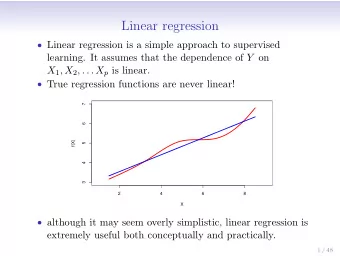
Linear regression • Linear regression is a simple approach to supervised learning. It assumes that the dependence of Y on X 1 , X 2 , . . . X p is linear. • True regression functions are never linear! 7 6 f(X) 5 4 3 2 4 6 8 X 1 / 48

Linear regression • Linear regression is a simple approach to supervised learning. It assumes that the dependence of Y on X 1 , X 2 , . . . X p is linear. • True regression functions are never linear! 7 6 f(X) 5 4 3 2 4 6 8 X • although it may seem overly simplistic, linear regression is extremely useful both conceptually and practically. 1 / 48

Linear regression for the advertising data Consider the advertising data shown on the next slide. Questions we might ask: • Is there a relationship between advertising budget and sales? • How strong is the relationship between advertising budget and sales? • Which media contribute to sales? • How accurately can we predict future sales? • Is the relationship linear? • Is there synergy among the advertising media? 2 / 48

Advertising data 25 25 25 20 20 20 Sales 15 Sales 15 Sales 15 10 10 10 5 5 5 0 50 100 200 300 0 10 20 30 40 50 0 20 40 60 80 100 TV Radio Newspaper 3 / 48

Simple linear regression using a single predictor X . • We assume a model Y = β 0 + β 1 X + � , where β 0 and β 1 are two unknown constants that represent the intercept and slope , also known as coe ffi cients or parameters , and � is the error term. • Given some estimates ˆ β 0 and ˆ β 1 for the model coe ffi cients, we predict future sales using y = ˆ β 0 + ˆ ˆ β 1 x, where ˆ y indicates a prediction of Y on the basis of X = x . The hat symbol denotes an estimated value. 4 / 48

Estimation of the parameters by least squares y i = ˆ β 0 + ˆ • Let ˆ β 1 x i be the prediction for Y based on the i th value of X . Then e i = y i − ˆ y i represents the i th residual 5 / 48

Estimation of the parameters by least squares y i = ˆ β 0 + ˆ • Let ˆ β 1 x i be the prediction for Y based on the i th value of X . Then e i = y i − ˆ y i represents the i th residual • We de fi ne the residual sum of squares (RSS) as RSS = e 2 1 + e 2 2 + · · · + e 2 n , or equivalently as RSS = ( y 1 − ˆ β 0 − ˆ β 1 x 1 ) 2 +( y 2 − ˆ β 0 − ˆ β 1 x 2 ) 2 + . . . +( y n − ˆ β 0 − ˆ β 1 x n ) 2 . 5 / 48

Estimation of the parameters by least squares y i = ˆ β 0 + ˆ • Let ˆ β 1 x i be the prediction for Y based on the i th value of X . Then e i = y i − ˆ y i represents the i th residual • We de fi ne the residual sum of squares (RSS) as RSS = e 2 1 + e 2 2 + · · · + e 2 n , or equivalently as RSS = ( y 1 − ˆ β 0 − ˆ β 1 x 1 ) 2 +( y 2 − ˆ β 0 − ˆ β 1 x 2 ) 2 + . . . +( y n − ˆ β 0 − ˆ β 1 x n ) 2 . • The least squares approach chooses ˆ β 0 and ˆ β 1 to minimize the RSS. The minimizing values can be shown to be � n i =1 ( x i − ¯ x )( y i − ¯ y ) ˆ β 1 = , � n x ) 2 i =1 ( x i − ¯ ˆ y − ˆ β 0 = ¯ β 1 ¯ x, y ≡ 1 � n x ≡ 1 � n where ¯ i =1 y i and ¯ i =1 x i are the sample n n means. 5 / 48

Example: advertising data 25 20 Sales 15 10 5 0 50 100 150 200 250 300 TV The least squares fi t for the regression of sales onto TV . In this case a linear fi t captures the essence of the relationship, although it is somewhat de fi cient in the left of the plot. 6 / 48

Assessing the Accuracy of the Coe ffi cient Estimates • The standard error of an estimator re fl ects how it varies under repeated sampling. We have � 1 σ 2 x 2 2 = 2 = σ 2 ¯ � SE(ˆ SE(ˆ β 1 ) β 0 ) n + x ) 2 , , � n � n i =1 ( x i − ¯ i =1 ( x i − ¯ x ) 2 where σ 2 = Var( � ) 7 / 48

Assessing the Accuracy of the Coe ffi cient Estimates • The standard error of an estimator re fl ects how it varies under repeated sampling. We have � 1 σ 2 x 2 2 = 2 = σ 2 ¯ � SE(ˆ SE(ˆ β 1 ) β 0 ) n + x ) 2 , , � n � n i =1 ( x i − ¯ i =1 ( x i − ¯ x ) 2 where σ 2 = Var( � ) • These standard errors can be used to compute con fi dence intervals. A 95% con fi dence interval is de fi ned as a range of values such that with 95% probability, the range will contain the true unknown value of the parameter. It has the form β 1 ± 2 · SE(ˆ ˆ β 1 ) . 7 / 48

Con fi dence intervals — continued That is, there is approximately a 95% chance that the interval � � β 1 − 2 · SE(ˆ ˆ β 1 ) , ˆ β 1 + 2 · SE(ˆ β 1 ) will contain the true value of β 1 (under a scenario where we got repeated samples like the present sample) 8 / 48

Con fi dence intervals — continued That is, there is approximately a 95% chance that the interval � � β 1 − 2 · SE(ˆ ˆ β 1 ) , ˆ β 1 + 2 · SE(ˆ β 1 ) will contain the true value of β 1 (under a scenario where we got repeated samples like the present sample) For the advertising data, the 95% con fi dence interval for β 1 is [0 . 042 , 0 . 053] 8 / 48