Regression Regression is a predictive method (like the nearest - PDF document
Regression Regression is a predictive method (like the nearest neighbour algorithm) The approach is to try to describe a dependent variable in terms of one or more independent variables Regression can be used with both quantitative
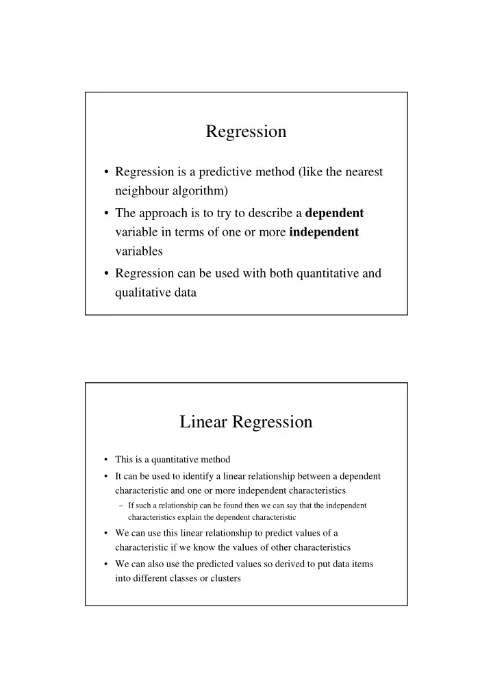
Regression • Regression is a predictive method (like the nearest neighbour algorithm) • The approach is to try to describe a dependent variable in terms of one or more independent variables • Regression can be used with both quantitative and qualitative data Linear Regression • This is a quantitative method • It can be used to identify a linear relationship between a dependent characteristic and one or more independent characteristics – If such a relationship can be found then we can say that the independent characteristics explain the dependent characteristic • We can use this linear relationship to predict values of a characteristic if we know the values of other characteristics • We can also use the predicted values so derived to put data items into different classes or clusters
The Linear Regression Model • The basic model deals with the case where we have just one independent variable or characteristic, X, which explains a dependent variable or characteristic, Y Given n pairs of observations for the dependent and independent variables • (x i , y i ) we can relate them to each other with a regression function = α + β + ε y x i i i That is, a straight line where ε i absorbs the divergence from the straight line, • or residual, for each pair of observations • The regression function is a combination of the residuals and the regression line (or approximation) = α + β y x ˆ i i Fitting the Model to the Data • To find the “best” regression line we need to find the “best” overall values for α and β • That is, the values which minimise the combined error contained in all the residuals • We can do this using the method of least squares which minimises the sum of the squares of the residuals • We find that σ α = µ − βµ β = y r X Y ( , ) y x σ x
Residual Analysis I The residuals, ε i , can tell us a lot about how well our linear model describes the • dependent variable, Y, in terms of the independent variable, X Having found the best values for α and β the sum of the residuals will be zero • because the errors will be equally spread either side (positive and negative) of the regression line but there may still be a pattern in the sign or magnitude of the residuals with respect to certain subsets of the observed values • Such patterns would indicate that our model may be over-simplistic • The residuals will be uncorrelated with both X and Y overall but this does not mean that they will be uncorrelated with all subsets of the observed values • Where subset correlations exist we have evidence that our model could be improved upon Residual Analysis II • Finally, although we know that the method of least squares has provided the best linear fit to our observed data, we don’t know how good this linear fit is – our observed data may not be linear • Consider the following relation that follows directly from the regression line ∑ ∑ ∑ − = − + − y y y y y y 2 2 2 ˆ ˆ ( ) ( ) ( ) i i i i • In words it is saying that the total sum of squares in the observations is equal the sum of squares of the regression (approximation) plus the sum of squares of the errors
Residual Analysis III If we divide these deviances by the number of observations, n , we will get • = + Var Y Var Y ˆ Var E ( ) ( ) ( ) • That is, the variance in the dependent variable comes from the variance explained by the regression line and the residual variance Var Y ˆ Var E • Consider now ( ) ( ) R = = − 2 1 Var Y Var Y ( ) ( ) • This is the square of the linear correlation coefficient and will by 0 when the regression line is constant (the gradient is 0) and it will be 1 when the regression line is a perfect fit (the residuals are 0) So the closer R 2 is to 1 the better our regression model is • Logistic Regression • This is a qualitative method • The dependent variable is normally binary and taken to mean presence or absence of a certain characteristic • We shall return to it when we cover artificial neural networks which are capable of handling non-linear relationships as well as linear ones
Recommend
More recommend
Explore More Topics
Stay informed with curated content and fresh updates.
