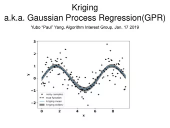
Kernel Methods for Regression Support Vector Regression Gaussian - PowerPoint PPT Presentation

MACHINE LEARNING MACHINE LEARNING MACHINE LEARNING Kernel Methods for Regression Support Vector Regression Gaussian Mixture Regression Gaussian Process Regression 1

MACHINE LEARNING – 2012 MACHINE LEARNING MACHINE LEARNING Problem Statement Predict given input through a non-linear function : y x f    y f x   i i Estimate that best predict set of training points , ? f x y  1,... i M y 3 y 2 y 4 y 1 y 1 2 3 4 x x x x x 2

MACHINE LEARNING – 2012 MACHINE LEARNING MACHINE LEARNING Non-linear regression and the Kernel Trick Non-Linear regression: Fit data with a function that is not linear in the parameters    x   ; ; : parameters of the function y f Non-parametric regression: use the data to determine the parameters of the function so that the problem can be again phrased as a linear regression problem. Kernel Trick: Send data in feature space with non-linear function and perform linear regression in feature space      i , y k x x i i i x : datapoints, k: kernel fct. 3

MACHINE LEARNING – 2012 MACHINE LEARNING MACHINE LEARNING Data-driven Regression Good prediction depends on the choice of datapoints. Blue: true function y Red: estimated function x 5

MACHINE LEARNING – 2012 MACHINE LEARNING MACHINE LEARNING Data-driven Regression Good prediction depends on the choice of datapoints. The more datapoints, the better the fit. Computational costs increase dramatically with number of datapoints Blue: true function y Red: estimated function x 6

MACHINE LEARNING – 2012 MACHINE LEARNING MACHINE LEARNING Kernel methods for regression Several methods in ML for performing non-linear regression. Differ in the objective function, in the amount of parameters. Gaussian Process Regression (GPR) uses all datapoints Blue: true function y Red: estimated function x 7

MACHINE LEARNING – 2012 MACHINE LEARNING MACHINE LEARNING Kernel methods for regression Several methods in ML for performing non-linear regression. Differ in the objective function, in the amount of parameters. Gaussian Process Regression (GPR) uses all datapoints Support Vector Regression (SVR) picks a subset of datapoints (support vectors) Blue: true function y Red: estimated function x 8

MACHINE LEARNING – 2012 MACHINE LEARNING MACHINE LEARNING Kernel methods for regression Several methods in ML for performing non-linear regression. Differ in the objective function, in the amount of parameters. Gaussian Process Regression (GPR) uses all datapoints Support Vector Regression (SVR) picks a subset of datapoints (support vectors) Gaussian Mixture Regression (GMR) generates a new set of datapoints (centers of Gaussian functions) Blue: true function y Red: estimated function x 9

MACHINE LEARNING – 2012 MACHINE LEARNING MACHINE LEARNING Kernel methods for regression   ,    N , y f x x y D eterministic regressive model           2 , with 0, Probabilistic regressive model y f x N Build an estimate of the noise model and then compute f directly (Support Vector Regression) y x 10

MACHINE LEARNING – 2012 MACHINE LEARNING MACHINE LEARNING Support Vector Regression 11

MACHINE LEARNING – 2012 MACHINE LEARNING MACHINE LEARNING Support Vector Regression (SVR)    Assume a nonlinear mapping , s.t. . f y f x   i i How to estimate to best predict the pair of training points , ? f x y  1,... i M How to generalize the support vector machine framework for classification to estimate continuous functions? 1. Assume a non-linear mapping through feature space and then perform linear regression in feature space Supervised learning – minimizes an error function. 2.  First determine a way to measure error on testing set in the linear case! 12

MACHINE LEARNING – 2012 MACHINE LEARNING MACHINE LEARNING Support Vector Regression b is estimated as in SVR through   least-square regression on    T Assume a linear mapping , s.t. . f y f x w x b support vectors; hence we omit it from the rest of the developments .   1,... i i How to estimate and to best predict the pair of training points , ? w b x y  i M    y f x Measure the error on prediction x 13

MACHINE LEARNING – 2012 MACHINE LEARNING MACHINE LEARNING Support Vector Regression  Set an upper bound on the error and consider as correctly classified all points    such that ( ) , f x y Penalize only datapoints that are +𝜁  not contained in the -tube. −𝜁 x 14

MACHINE LEARNING – 2012 MACHINE LEARNING MACHINE LEARNING Support Vector Regression The  -margin is a measure of the   y wx b width of the  -insensitive tube and hence of the precision of the regression. A small || w || corresponds to a  small slope for f . In the linear case, f is more horizontal.  X  -margin 15

MACHINE LEARNING – 2012 MACHINE LEARNING MACHINE LEARNING Support Vector Regression A large || w || corresponds to a large   y wx b slope for f . In the linear case, f is more vertical. The flatter the slope of the function f, the larger the  margin   To maximize the margin, we must minimize the norm of w.  X  -margin 16

MACHINE LEARNING – 2012 MACHINE LEARNING MACHINE LEARNING Support Vector Regression This can be rephrased as a constraint-based optimization problem of the form: Need to penalize points outside 1 the  -insensitive 2 minimize w tube. 2      i , w x b y  i  subject to      i , y w x b i  𝜁   1,... i M 17

MACHINE LEARNING – 2012 MACHINE LEARNING MACHINE LEARNING Support Vector Regression    * Introduce slack variables , , 0 : C i i Need to penalize points outside the  -insensitive   1 C M  2    * minimize + w tube. i i 2 M  i 1        i , w x b y i  i   i       i *  subject to ,  y w x b i * i 𝜁  i     *  0, 0  i i 18

MACHINE LEARNING – 2012 MACHINE LEARNING MACHINE LEARNING Support Vector Regression    * Introduce slack variables , , 0 : C i i All points outside the  -tube become   1 C M  2    Support Vectors * minimize + w i i 2 M  1 i        i , w x b y i  i   i       *  i subject to ,  y w x b i * 𝜁 i  i     *  0, 0  i i We now have the solution to the linear regression problem. How to generalize this to the nonlinear case? 19

MACHINE LEARNING – 2012 MACHINE LEARNING MACHINE LEARNING Support Vector Regression Lift x into feature space and then perform linear regression in feature space. Linear Case:      , y f x w x b     Non-Linear Case: x x     x x            , y f x w x b w lives in feature space! 20

MACHINE LEARNING – 2012 MACHINE LEARNING MACHINE LEARNING Support Vector Regression In feature space, we obtain the same constrained optimization problem:   1 C M  2    * minimize + w i i 2 M  1 i           i , w x b y i  i           *  i subject to , y w x b i i      *  0, 0  i i 21

MACHINE LEARNING – 2012 MACHINE LEARNING MACHINE LEARNING Support Vector Regression Again, we can solve this quadratic problem by introducing sets of Lagrange multipliers and writing the Lagrangian : Lagrangian = Objective function + l * constraints     M M 1 C C     2            * * * L , , *, = + w b w i i i i i i 2 M M   1 1 i i     M           i , y w x b i i i  i 1     M           * * i , y w x b i i i  1 i 22

MACHINE LEARNING – 2012 MACHINE LEARNING MACHINE LEARNING Support Vector Regression Requiring that the partial derivatives are all zero    L M       * 0;  i i b  i 1      M L         * i 0; w x  i i w  i 1  L C           * * 0     i i * i M And replacing in the primal Lagrangian, we get the Dual optimization problem:        1 M         * * i j ,  k x x i i j j  2  i j , 1  max       M M     *         , * * i y  i i i i    1 1 i i     M  C         * * i subject to 0 and , 0,  i i i i   M  i 1 23