State Space Gaussian Processes with Non-Gaussian Likelihoods Hannes - PowerPoint PPT Presentation
State Space Gaussian Processes with Non-Gaussian Likelihoods Hannes Nickisch 1 Arno Solin 2 Alexander Grigorievskiy 2 , 3 1 Philips Research, 2 Aalto University, 3 Silo.AI ICML2018 July 13, 2018 Outline Gaussian Processes Temporal GPs as
State Space Gaussian Processes with Non-Gaussian Likelihoods Hannes Nickisch 1 Arno Solin 2 Alexander Grigorievskiy 2 , 3 1 Philips Research, 2 Aalto University, 3 Silo.AI ICML2018 July 13, 2018
Outline Gaussian Processes Temporal GPs as stochastic differential equations (SDEs) Learning and inference with Gaussian Likelihoods Speeding up computation of state space model parameters Non-Gaussian likelihoods Approximate inference algorithms Computational primitives and how to compute them Experiments Non-Gaussian State Space GPs Poster #151 Nickisch, Solin, Grigorievskiy 2/ 14
Gaussian Processes (GPs) Def: Gaussian Process (GP) is a stochastic process where for any inputs t all corresponding outputs y are distributed as y ∼ N ( m ( t ) , K ( t , t | θ )) . Denoted: f ( t ) ∼ GP ( m ( t ) , k ( t , t ′ | θ )) ◮ Used as a prior over continuous functions in statistical models ◮ Properties (e.g. smoothness) are determined by the covariance function k ( t , t ′ | θ ) Non-Gaussian State Space GPs Poster #151 Nickisch, Solin, Grigorievskiy 3/ 14
Temporal Gaussian Processes ◮ Input data is 1-D, usually time ◮ Fully probabilistic (Bayesian) approach ◮ Conveniently combining structural Challenges: components by covariance operations ◮ Large datasets ◮ Non-Gaussian likelihoods ◮ Applicability for unevenly sampled data Non-Gaussian State Space GPs Poster #151 Nickisch, Solin, Grigorievskiy 4/ 14
Temporal Gaussian Processes ◮ Input data is 1-D, usually time ◮ Fully probabilistic (Bayesian) approach ◮ Conveniently combining structural Challenges: components by covariance operations ◮ Large datasets ◮ Non-Gaussian likelihoods ◮ Applicability for unevenly sampled data Non-Gaussian State Space GPs Poster #151 Nickisch, Solin, Grigorievskiy 4/ 14
GP as a Stochastic Differential Equation (SDE) Addressing challenge 1 Given a 1-D time series: { y i , t i } N i = 1 ◮ Gaussian Process ◮ Equivalent Stochastic Differential model: Equation (SDE) [3] d f ( t ) f ( t ) ∼ GP ( m ( t ) , k ( t , t ′ )) = Ff ( t ) + Lw ( t ); f 0 ∼ N ( 0 , P ∞ ) GP prior d t n n � y | f ∼ P ( y i | f ( t i )) Likelihood � y | f ∼ P ( y i | Hf ( t i )) i = 1 i = 1 ◮ Latent Posterior: ◮ f ( t ) = Hf ( t ) ◮ w ( t ) - multidimensional white noise Q ( f | D ) = ◮ F , L , H , P ∞ are determined from the � m + K α , ( K − 1 + W ) − 1 � � � N f covariance K [3] � Non-Gaussian State Space GPs Poster #151 Nickisch, Solin, Grigorievskiy 5/ 14
GP as a Stochastic Differential Equation (SDE) Addressing challenge 1 Given a 1-D time series: { y i , t i } N i = 1 ◮ Gaussian Process ◮ Equivalent Stochastic Differential model: Equation (SDE) [3] d f ( t ) f ( t ) ∼ GP ( m ( t ) , k ( t , t ′ )) = Ff ( t ) + Lw ( t ); f 0 ∼ N ( 0 , P ∞ ) GP prior d t n n � y | f ∼ P ( y i | f ( t i )) Likelihood � y | f ∼ P ( y i | Hf ( t i )) i = 1 i = 1 ◮ Latent Posterior: ◮ f ( t ) = Hf ( t ) ◮ w ( t ) - multidimensional white noise Q ( f | D ) = ◮ F , L , H , P ∞ are determined from the � m + K α , ( K − 1 + W ) − 1 � � � N f covariance K [3] � Non-Gaussian State Space GPs Poster #151 Nickisch, Solin, Grigorievskiy 5/ 14
Inference and Learning with Gaussian likelihood Gaussian likelihood: P ( y i | f ( t i )) = N ( y i | f ( t i ) , σ 2 n I ) ◮ Solve SDE between time points ◮ Posterior parameters: (equivalent discrete time model): W = σ − 2 I n f i = A i − 1 f i − 1 + q i − 1 ; q i − 1 ∼ N ( 0 , Q i − 1 ) α = ( K + W − 1 ) − 1 ( y − m ) ǫ n ∼ N ( 0 , σ 2 y i = Hf i + ǫ i ; n ) ◮ Parameters of the discrete ◮ Evidence: model: log Z GPR = − 1 A i = A [∆ t i ] = e ∆ t i F , 2 α ⊤ ( y − m ) Q i = P ∞ − A i P ∞ A ⊤ − 1 2 log | K + W − 1 | − N i 2 log ( 2 πσ 2 n ) ◮ Inference and learning by Kalman FIlter (KF) and ıve approach has O ( N 3 ) ◮ The na¨ Rauch-Tung-Striebel (RTS) complexity smoother in O ( N ) complexity Non-Gaussian State Space GPs Poster #151 Nickisch, Solin, Grigorievskiy 6/ 14
Inference and Learning with Gaussian likelihood Gaussian likelihood: P ( y i | f ( t i )) = N ( y i | f ( t i ) , σ 2 n I ) ◮ Solve SDE between time points ◮ Posterior parameters: (equivalent discrete time model): W = σ − 2 I n f i = A i − 1 f i − 1 + q i − 1 ; q i − 1 ∼ N ( 0 , Q i − 1 ) α = ( K + W − 1 ) − 1 ( y − m ) ǫ n ∼ N ( 0 , σ 2 y i = Hf i + ǫ i ; n ) ◮ Parameters of the discrete ◮ Evidence: model: log Z GPR = − 1 A i = A [∆ t i ] = e ∆ t i F , 2 α ⊤ ( y − m ) Q i = P ∞ − A i P ∞ A ⊤ − 1 2 log | K + W − 1 | − N i 2 log ( 2 πσ 2 n ) ◮ Inference and learning by Kalman FIlter (KF) and ıve approach has O ( N 3 ) ◮ The na¨ Rauch-Tung-Striebel (RTS) complexity smoother in O ( N ) complexity Non-Gaussian State Space GPs Poster #151 Nickisch, Solin, Grigorievskiy 6/ 14
Fast computation of A i and Q i by interpolation Problem: ◮ Use 4-point interpolation: ◮ When there are many ∆ t i A ≈ c 1 A j − 1 + c 2 A j + parameters computation c 3 A j + 1 + c 4 A j + 2 . can be slow Coefficients { c i } 4 i = 1 are Solution: efficiently computable ◮ ψ : s �→ e s X is smooth mean ± min/max errors visualized. mapping, hence 10 Na¨ ıve interpolation (similar to State space 8 State space ( K = 2000 ) Evaluation time (s) KISS-GP [4]) State space ( K = 10 ) 6 ◮ Evaluate ψ on an 4 equispaced grid 2 s 1 , s 2 , .., s K , where 0 s j = s 0 + j · ∆ s 5 10 15 20 · 10 3 Number of training inputs, n Non-Gaussian State Space GPs Poster #151 Nickisch, Solin, Grigorievskiy 7/ 14
Non-Gaussian Likelihoods Addressing challenge 2 Posterior as a Gaussian approximation: � m + K α , ( K − 1 + W ) − 1 � � � Q ( f | D ) = N f Laplace Approximation ◮ log P ( f | D ) ∼ log P ( f | y ) + log P ( f | t ) ◮ Laplace approximation (LA) ◮ Find the mode ˆ f of this function ◮ Variational Bayes (VB) by Newton method ◮ Direct Kullback-Liebler ◮ Hessian at the mode ˆ f is minimization (KL) precision W = − ∂ 2 log P (ˆ f | t ) ◮ Assumed Density Filtering (ADF) � a.k.a. single sweep Expectation ◮ log Z LA = − 1 α ⊤ mvm K ( α ) + Propagation (EP) 2 � i log P ( y i | ˆ ld K ( W ) − 2 � f i ) Non-Gaussian State Space GPs Poster #151 Nickisch, Solin, Grigorievskiy 8/ 14
Computational Primitives The following computational primitives allow to cast the covariance approximation in more generic terms: ◮ Linear system solving: solve K ( W , r ) := ( K + W − 1 ) − 1 r ◮ Matrix-vector multiplications: mvm K ( r ) := Kr ◮ Log-determinants: ld K ( W ) := log | B | with well-conditioned 1 1 2 K W B = I + W 2 ◮ Predictions need latent mean E [ f ∗ ] and variance V [ f ∗ ] Non-Gaussian State Space GPs Poster #151 Nickisch, Solin, Grigorievskiy 9/ 14
Tackling computational primitives Using state space from of temporal GPs SpInGP: ◮ The first two computational primitives are calculated using SpInGP [5] approach: ◮ Idea is: using state space form compose the inverse of the covariance matrix, which turns out to be block-tridiagonal KF and RTS Smoothing: ◮ The last two primitives are solved by Kalman filtering and RTS smoothing ◮ Predictions are computed by primitive 4 and then by propagation through likelihood Comments: ◮ Derivatives of computational primitives, required for learning, are computed in a similar way ◮ SpInGP involves computations with block-tridiagonal matrices. These computations are similar to KF and RTS smoothing (see [1] Appendix) Non-Gaussian State Space GPs Poster #151 Nickisch, Solin, Grigorievskiy 10/ 14
Experiments 2-3 Experiments are designed to emphasize the paper findings and statements 1. A robust regression (Student’s t likelihood) study example with n = 34 , 154 observations 2. Numerical effects in non-Gaussian likelihoods Non-Gaussian State Space GPs Poster #151 Nickisch, Solin, Grigorievskiy 11/ 14
Experiment 4 ◮ A new interesting data set with commercial airline accidents dates scraped from Wikipedia [6] ◮ Accidents over the time-span of ∼ 100 years, n = 35 , 959 days ◮ We model the accident intensity as a Log Gaussian Cox process (Poisson likelihood) ◮ The GP prior is set up as: k ( t , t ′ ) = k Mat. ( t , t ′ ) + k per. ( t , t ′ ) k Mat. ( t , t ′ ) Non-Gaussian State Space GPs Poster #151 Nickisch, Solin, Grigorievskiy 12/ 14
Conclusions ◮ This paper brings together research done in state space GPs and non-Gaussian approximate inference ◮ We improve stability and provide additional speed-up by fast computations of the state space model parameters ◮ We provide unifying code for all approches in GPML toolbox v. 4.2 [7] ◮ Visit our poster: #151 Non-Gaussian State Space GPs Poster #151 Nickisch, Solin, Grigorievskiy 13/ 14
Recommend
More recommend
Explore More Topics
Stay informed with curated content and fresh updates.
