Determining the PSF over the Full FoV of LSST using Anisotropic - PowerPoint PPT Presentation

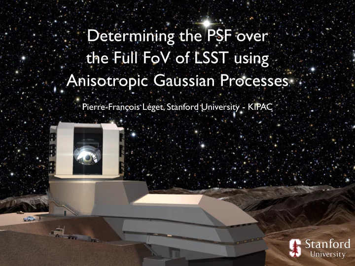
Determining the PSF over the Full FoV of LSST using Anisotropic Gaussian Processes Pierre-François Léget, Stanford University - KIPAC

Gaussian process (GP) interpolation: Gaussian processes are a non-parametric way to • interpolate data Interpolation is driven by the correlation function (aka • kernel) described by «hyperparameters»; for example, amplitude of the fluctuations • correlation length • … • Basic steps in GP interpolation: • Choose a correlation function (kernel) • Fit hyperparameters • Compute interpolated values • Best Linear Unbiased Estimator. • ➡ GP may be optimal interpolation method for atmospheric PSF parameters 2

Gaussian process (GP) interpolation: Atmosphere introduces anisotropy • Davis et al. 2016 (preferential direction) in spatial variation of PSF’s parameters It means that the spacial variation in the • case of a anisotropic gaussian random field are characterized by a 2D 2-point Anisotropic Anisotropic correlation function Gaussian random field Correlation function • For the anisotropic GP , 4 hyperparameters: • Amplitude of spatial fluctuations • Correlation length « g 1 » • Same parametrization as « g 2 » in shape measurement • • Need to estimate those hyperparameters to predict the PSF over the FoV using GP 3

Realistic simulation of atmospheric PSF Generated realistic atmospheric PSFs across • FoV using GalSim. Phase screens generated with Von Kármán • power spectrum (Kolmogorov with finite outer scale). Each screen corresponds to different wind • speed & direction, & outer scale. 6 screens between 0.1 km & 15 km • Wind speed increases in with altitude • Dominant wind direction • Assumes 30-sec exposures for an LSST -like • aperture and obscuration (no optical PSF). 20 000 stars on LSST FoV: • fit with elliptical Kolmogorov profile. • Fit parameters: size, g 1 , g 2. • 4

Interpolation of atmospheric PSF Two interpolations are made on simulation: • GP interpolation with anisotropic Von-Kármán kernel (over the full FoV) • Second-order polynomial interpolation (for each CCD) • 80% of stars are used for training (16 000). • 20% of stars are kept for validation (4 000). • 5

Results: Anisotropic 2-point correlation function fit on PSF parameters Compute for each PSF’s parameter the • anisotropic 2-point correlation function (left plots) Estimate the covariance matrix with an • internal method (bootstrapping) Fit each measured anisotropic 2-point • correlation function with an anisotropic Von-Karman correlation function. 6

Results: Gaussian processes with 2nd order polynomial interpolation (per CCD) anisotropic Von-Kármán kernel (FoV) For each interpolation, we compute “Rowe statistics”, which are ingredients • in the calculation of the systematic error in the shear correlation function due to errors in the PSF model. • Rowe statistics computed for stars in validation sample (4 000 stars). • Rowe statistics are lower for GP than for polynomial interpolation by a factor of ~3 for all 𝜍 statistics • Next step: apply to real data (DES) 7