Dynamical Approach to Dynamical Approach to Nonlinear Ensemble Data - PowerPoint PPT Presentation
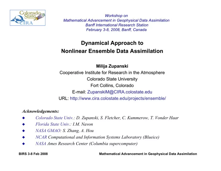
Workshop on Mathematical Advancement in Geophysical Data Assimilation Banff International Research Station February 3-8, 2008, Banff, Canada Dynamical Approach to Dynamical Approach to Nonlinear Ensemble Data Assimilation Nonlinear Ensemble
Workshop on Mathematical Advancement in Geophysical Data Assimilation Banff International Research Station February 3-8, 2008, Banff, Canada Dynamical Approach to Dynamical Approach to Nonlinear Ensemble Data Assimilation Nonlinear Ensemble Data Assimilation Milija Zupanski Milija Zupanski Cooperative Institute for Research in the Atmosphere Cooperative Institute for Research in the Atmosphere Colorado State University Colorado State University Fort Collins, Colorado Fort Collins, Colorado E-mail: ZupanskiM@CIRA.colostate.edu E-mail: ZupanskiM@CIRA.colostate.edu URL: URL: http://www.cira.colostate.edu/projects/ensemble/ Acknowledgements: Colorado State Univ.: D. Zupanski, S. Fletcher, C. Kummerow, T. Vonder Haar Florida State Univ.: I.M. Navon NASA GMAO: S. Zhang, A. Hou NCAR Computational and Information Systems Laboratory (Blueice) NASA Ames Research Center (Columbia supercomputer) BIRS 3-8 Feb 2008 Mathematical Advancement in Geophysical Data Assimilation
Overview Dynamics and nonlinearity in data assimilation A prototype for dynamical ensemble DA algorithm: MLEF Example 1: MLEF + 1-D soil model Example 2: MLES + NASA GEOS-5 global model + precipitation Example 3: MLEF + WRF regional model Conclusion and Future work BIRS 3-8 Feb 2008 Mathematical Advancement in Geophysical Data Assimilation
Dynamics and nonlinearity in data assimilation (1) Create dynamically consistent analysis DA is a dynamic-stochastic problem - Dynamics reduces the number of degrees of freedom (DOF) - Dynamics has a “localization” capability Dynamical requirement: - Analysis and uncertainties are in dynamical balance: x a = x f + Δ x a ; P a 1/2 - Easier problem: If the first-guess is in balance, need only to make sure that the analysis correction is in dynamical balance Possible solutions: 1 - Stage 1 : Get analysis without enforcing dynamical balance; Stage 2 : filter the noise after analysis to produce the balanced state 2 - Get balanced analysis by enforcing dynamical balance in DA BIRS 3-8 Feb 2008 Mathematical Advancement in Geophysical Data Assimilation
Dynamics and nonlinearity in data assimilation (2) Address nonlinearity in prediction and observations Fundamental theoretical development in DA is based on linear assumptions - Kalman Filtering, Best Linear Unbiased Estimate (BLUE) Real world is nonlinear - Physical processes (i.e. clouds, precipitation) - Observation operators (remote sensing, physics related observations) Typical solutions: - Direct Use linear analysis solution + insert nonlinear operators into linear solution - Indirect Solution of nonlinear analysis problem by minimizing nonlinear cost function BIRS 3-8 Feb 2008 Mathematical Advancement in Geophysical Data Assimilation
Forecast error covariance Forecast error covariance In DA the (square-root) forecast error covariance defines the uncertainty space in which the analysis is corrected x a � x f = P f 1 + w 2 p f 2 + � + w N p f 1/2 w = w 1 p f N 1) The analysis increment is in dynamical balance if the column-vectors of the square-root forecast error covariance are in dynamical balance 2) The analysis is in dynamical balance if the first guess and the analysis increment are in dynamical balance • How well the dynamical balance can be enforced in P f ? • What is the impact of (unbalanced) P f in cycling of DA? BIRS 3-8 Feb 2008 Mathematical Advancement in Geophysical Data Assimilation
Means for ensuring the dynamical balance Create balanced first guess Create balanced forecast error perturbations - the dynamical balance in P f can be enforced by initiating DA with balanced initial conditions and balanced initial ensemble perturbations - if the initial ensemble perturbations are not in balance, the noise can remain in short-range forecast used to calculate the first guess, eventually contaminating the next cycle analysis - enforcing the dynamical balance during the analysis is more beneficial then enforcing it after the analysis is completed - analysis perturbations have to be projected on dynamically consistent directions that will not create a spin-up of the model forecast - cycling of data assimilation has beneficial impact on dynamical balance BIRS 3-8 Feb 2008 Mathematical Advancement in Geophysical Data Assimilation
Addressing the nonlinearities and dynamical Addressing the nonlinearities and dynamical balance using the Maximum Likelihood balance using the Maximum Likelihood Ensemble Filter (MLEF) Ensemble Filter (MLEF) MLEF developed as a nonlinear extension to Kalman Filter - First-guess obtained using a nonlinear model forecast - Square-root forecast error covariance columns defined as dynamically balanced span-vectors of analysis correction subspace - Nonlinear analysis obtained using iterative minimization of the cost function defined over the analysis correction subspace - Full-rank or reduced-rank method - Could be extended to non-Gaussian PDFs - Not sample based References : Zupanski 2005; Zupanski and Zupanski 2006; Zupanski et al. 2008; Fletcher and Zupanski 2007a, 2007b) BIRS 3-8 Feb 2008 Mathematical Advancement in Geophysical Data Assimilation
Mathematical formulation of the MLEF Mathematical formulation of the MLEF 1) Initial state and uncertainty : Define an initial state and a subspace (span-vectors) 0 = x 0 + u i 0 ; � � ( i = 1 , … ,N E ) x 0 , span { u i 0 } x i � � 2) Prediction : Transport the uncertainty span-vectors in time by a prediction model x t = M ( x t � 1 ) t � 1 ) } t = M ( x t � 1 + u i � � t � 1 ) � M ( x t � 1 ) x t , span { u i t } u i � � x t + u i t = M ( x t � 1 + u i [ ] max P ( X | Y ) = min � ln P ( X | Y ) 3) Analysis : Maximum a posteriori estimate � � - Iterative minimization of cost function over the ensemble subspace t } span { u i � � y + v i = H ( x + u i ) } y = H ( x ) [ ] v i = H ( x + u i ) � H ( x ) span { v i } BIRS 3-8 Feb 2008 Mathematical Advancement in Geophysical Data Assimilation
Examples with MLEF Examples with MLEF MLEF with 1-D 1-point soil temperature model o - Nonlinear observation operators (fluxes) - 1 degree of freedom MLES with NASA GEOS-5 global model o - Assimilation of accumulated precipitation observations (nonlinear) - Smoother MLEF with regional WRF MODEL o - Linear observation operators, but poor geographical coverage - Hurricane simulation BIRS 3-8 Feb 2008 Mathematical Advancement in Geophysical Data Assimilation
Example 1: MLEF + 1-D soil model Example 1: (B. Rajkovic, B. Orescanin - Univ. Belgrade, Serbia) One-point nonlinear soil • � t = M ( � t � 1 ) => temperature model H 2 ( � ) � e a 1 ( � � � s ) ) H 1 ( � ) � � 4 Nonlinear observation operators => • � � a 2 1 DOF => 1 ensemble member • Dynamical method: For a system with 1 DOF, need 1 ensemble! Technically no solution exists with sampling methods. BIRS 3-8 Feb 2008 Mathematical Advancement in Geophysical Data Assimilation
Example 2: MLES + GEOS-5 + precipitation MLES + GEOS-5 + precipitation Example 2: (D. Zupanski, S. Zhang, A. Hou Hou) ) (D. Zupanski, S. Zhang, A. Goal : Assimilate multi-sensor precipitation observations (accumulated rainfall observations from TRMM and SSM/I) to improve precipitation analysis Update specific humidity to improve fit to the precipitation obs and pseudo data Other variables ( U,V,T,Ps ) are taken from the NASA G5DAS 3d-Var GSI analyses Model resolution : 2x2.5 degrees, 72 vertical levels (144x91x72), N S ~1,000,000 Assimilation : 6-hour assimilation cycle, 8 days of assimilation Method : Maximum Likelihood Ensemble Smoother (MLES) 32 ensembles Error covariance localization based on a modified local-domains approach (10x10 points in each local domain) BIRS 3-8 Feb 2008 Mathematical Advancement in Geophysical Data Assimilation
Assimilation results Assimilation results BIRS 3-8 Feb 2008 Mathematical Advancement in Geophysical Data Assimilation
Example 3: MLEF + WRF regional model MLEF + WRF regional model Example 3: Hurricane Katrina (landfall 12Z 29 AUG 2005): Hurricane Katrina (landfall 12Z 29 AUG 2005): Model resolution : 30 km horizontal, 28 vertical levels (75x70x28) 6-hour old boundary conditions from the NCEP GFS model Observations : NCAR upper-air and surface observations ( p s , T , q , u , v ) Assimilation : 6-hour interval, from 26 Aug 00Z - 31 Aug 00Z (5 days) Control variables : u , v , δ θ , δ Z , q v State vector dimension ~ 700,000 32 ensembles Error covariance localization based on a modified local-domains approach (23x25 points in each local domain) BIRS 3-8 Feb 2008 Mathematical Advancement in Geophysical Data Assimilation
Radiosonde and SYNOP Observations (at 12 UTC) 20 Radiosondes + 409 SYNOPs ~ 1000-3000 observations Irregular observation coverage: Mostly surface + over the land BIRS 3-8 Feb 2008 Mathematical Advancement in Geophysical Data Assimilation
Surface pressure in the MLEF and No-DA experiments 29 AUG 00 UTC (12-hour before landfall) NO-DA MLEF (no assimilation) (with assimilation) Data assimilation with MLEF improves the position and intensity of the hurricane BIRS 3-8 Feb 2008 Mathematical Advancement in Geophysical Data Assimilation
Recommend
More recommend
Explore More Topics
Stay informed with curated content and fresh updates.
