Reconst nstruct ruct Radio o Map with Automatic atically ally - PowerPoint PPT Presentation
Reconst nstruct ruct Radio o Map with Automatic atically ally Constru tructed cted Gaussia sian n Proces ess s for Localiz lizatio ation 01 | Background C O N T E N T 02 | Gaussian Process 03 | Kernel Selection 04 | Model
Reconst nstruct ruct Radio o Map with Automatic atically ally Constru tructed cted Gaussia sian n Proces ess s for Localiz lizatio ation
目 01 | Background C O N T E N T 02 | Gaussian Process 03 | Kernel Selection 录 04 | Model Ensemble 05 | Experiment
Page . Page . 3 0 P A R T Background 1 O N E
GPS : time consuming Power consuming Turn on meter Base station Signal strength
• a large outdoor • indoor localization use environment fingerprinting • sample thousands of • creating a radio map survey sites to construct a fine grain • Received Signal Strength radio map Indicators (RSSI) values obtained from multiple • a university usually access points (APs) needs hundred thousand training data
About one million sample data 20 square kilometers SJTU 3G 4G Yindu Road 3G 4G
0 P A R T Gaussian 2 Process T W O
Given a training set 𝐸 = 𝒚 𝑗 , 𝑧 𝑗 𝑗 = 1, … , 𝑜} How to calculate the output 𝑧 ∗ for a new input 𝑦 ∗ Linear regression? – Least Square Method Nonlinear regression? -- Gaussian Process
Rela elation onship ip to Lin inear ar Regr egression on • In logistic regression, the input to the sigmoid function is where are parameters. T f x b • A Gaussian process places a prior on the space of functions f directly, without parameterizing f. • Therefore, Gaussian processes are non-parametric • more general than standard regression the form not limited by a parametric form
Given a training set 𝐸 = 𝒚 𝑗 , 𝑧 𝑗 𝑗 = 1, … , 𝑜} How to calculate the output 𝑧 ∗ (RSS) for a new input 𝑦 ∗ ( longitude/latitude ) Assume 𝒛 = {𝑧 1 , 𝑧 2 , … , 𝑧 𝑜 } obey multivariate Gaussian Distribution 𝑧 1 ⋮ ~𝑂 0, 𝐿 → 𝒛~𝑂 0, 𝐿 𝑧 𝑜 Where
Definiti De nition n of GP GP • A Gaussian process any finite number of which have joint Gaussian distributions. f gp m k ( , ) • A Gaussian process is fully specified by its mean function m(x) and covariance function k(x,x ’). • Two things to define our GP: • choose a form for the mean function. • choose a form for the covariance function
For new input data y* joint distribution defined as:
Get conditional distribution : Mean and variance:
Tun une Hyper-Par aram ameters Hyper-parameters: : Maxlimum: Maxlimum the log likelihood: (conjugate gradients)
Hype per-parameters The covariance function defines how smoothly the (latent) function f varies from a given x. SE kernel : 2 : overall vertical scale of variation of the latent value. 𝜏 𝑔 𝑚 : characteristic length-scale • short means the error bars can grow rapidly away from the data points. • large implies irrelevant features . 2 : noise variance 𝜏 𝑜
Hype per-parameters Different hyper parameters Bias & Variance trade off l eft with small 𝑚 right with large 𝑚
0 P A R T Kernel Selection 3 t h r e e
Squared Exponential Kernel Periodic Kernel Linear Kernel
( 1 ) ka + kb = ka(x, x′) + kb(x, x′ ) ( Summation ) ( 2 ) ka × kb = ka(x, x′) × kb(x, x′ ) ( Multiplication )
Automatic Mo Model Construction choosing the structural form of the kernel: a black art • Search over sums and products of kernels • Maximizing the BIC(M) • Show how any model be decomposed into different parts BIC trades off model fit and complexity
0 P A R T Model 4 F O U R Ensemble
Don’t Overfit! 1)average out biases Averaging multiple different 2)reduce the variance green lines should bring us 3)unlikely to overfit closer to the black line.
Linear regression SVR Gradient Tree Boosting Xgboost GP (RQ) GP (Compose) Rate Averaging Blending
0 Experiment P A R T 5 Results F I V E
Q&A P A R T S I X 6 0
Recommend


More recommend
Explore More Topics
Stay informed with curated content and fresh updates.