Optimization for Kernel Methods S. Sathiya Keerthi Yahoo! Research, - PDF document
Optimization for Kernel Methods S. Sathiya Keerthi Yahoo! Research, Burbank, CA, USA Kernel methods: Support Vector Machines (SVMs) Kernel Logistic Regression (KLR) Aim: To introduce a variety of optimization problems that arise in the
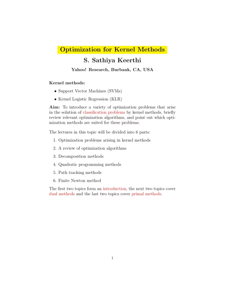
Optimization for Kernel Methods S. Sathiya Keerthi Yahoo! Research, Burbank, CA, USA Kernel methods: • Support Vector Machines (SVMs) • Kernel Logistic Regression (KLR) Aim: To introduce a variety of optimization problems that arise in the solution of classification problems by kernel methods, briefly review relevant optimization algorithms, and point out which opti- mization methods are suited for these problems. The lectures in this topic will be divided into 6 parts: 1. Optimization problems arising in kernel methods 2. A review of optimization algorithms 3. Decomposition methods 4. Quadratic programming methods 5. Path tracking methods 6. Finite Newton method The first two topics form an introduction, the next two topics cover dual methods and the last two topics cover primal methods. 1
Part I Optimization Problems Arising in Kernel Methods References: 1. B. Sch¨ olkopf and A. Smola, Learning with Kernels, MIT Press, 2002, Chapter 7, Pattern Recognition. 2
Kernel methods for Classification problems • Although kernel methods are used for a range of problems such as classification (binary/multiclass), regression, ordinal regres- sion, ranking and unsupervised learning, we will focus only on binary classification problems. • Training data: { x i , t i } n i =1 • x i ∈ R m is the i -th input vector. • t i ∈ { 1 , − 1 } is the target for x i , denoting the class to which the i -th example belongs; 1 denotes class 1 and − 1 denotes class 2. • Kernel methods transform x to a Reproducing Kernel Hilbert Space, H via φ : R m → H and then develop a linear classifier in that space: y ( x ) = w · φ ( x ) + b y ( x ) > 0 ⇒ x ∈ Class 1; y ( x ) < 0 ⇒ x ∈ Class 2 • The dot product in H , i.e., k ( x i , x j ) = φ ( x i ) · φ ( x j ) is called the Kernel function . All computations are done using k only. • Example: φ ( x ) is the vector of all monomials up to degree d on the components of x . For this example, k ( x i , x j ) = (1+ x i · x j ) d . This is the polynomial kernel function. Larger the value of d is, more flexible and powerful is the classifer function. • RBF kernel: k ( x i , x j ) = e − γ � x i − x j � 2 is another popular kernel function. Larger the value of γ is, more flexible and powerful is the classifer function. • Training problem: ( w, b ), which define the classifier are ob- tained by solving the following optimization problem: min w,b E = R + C L • L is the Empirical error defined as � L = l ( y ( x i ) , t i ) i l is a loss function that describes the discrepancy between the classifier output y ( x i ) and the target t i . 3
• Minimizing only L can lead to overfitting on the training data. The regularizer function R prefers simpler models and helps prevent overfitting. • The parameter C helps to establish a trade-off between R and L . C is a hyperparameter . (Other parameters such as d in the polynomial kernel and γ in the RBF kernel are also hyperpa- rameters .) All hyperparameters need to be tuned at a higher level. Some commonly used loss functions • SVM (Hinge) loss: l ( y, t ) = 1 − ty if ty < 1; 0 otherwise. • KLR (Logistic) loss: l ( y, t ) = − log(1 + exp( − ty )) • L 2 -SVM loss: l ( y, t ) = (1 − ty ) 2 / 2 if ty < 1; 0 • Modified Huber loss: l ( y, t ) is: 0 if ξ ≥ 0; ξ 2 / 2 if 0 < ξ < 2; and 2( ξ − 1) if ξ ≥ 2, where ξ = 1 − ty . 4
Margin based regularization • The margin between the planes defined by y ( x ) = ± 1 is 2 / � w � . Making the margin big is equivalent to making the function 2 � w � 2 small. R = 1 • This function is a very effective regularizing function. This is the natural regularizer associated with the RKHS. • Although there are other regularizers that have been considered in the literature, in these lectures I will restrict attention to only the optimization problems directly related to the above mentioned natural regularizer. Primal problem: 2 � w � 2 + C � min 1 i l ( y ( x i ) , t i ) 2 b 2 is also added in order to handle w and b Sometimes the term 1 uniformly. (This is also equivalent to ignoring b and instead adding a constant to the kernel function.) 5
Solution via Wolfe dual • w and y ( · ) have the representation: � � w = α i t i φ ( x i ) , y ( x ) = α i t i k ( x, x i ) i i • w could reside in an infinite dimensional space (e.g., in the case of the RBF kernel) and so we have to necessarily handle the solution via finite dimensional quantities such as the α i ’s. This is effectively done via the Wolfe dual (details will be covered in lectures on kernel methods by other speakers). SVM dual: (Convex quadratic program) min E ( α ) = 1 � i,j t i t j α i α j k ( x i , x j ) − � s . t . 0 ≤ α i ≤ C, � i α i i t i α i = 0 2 KLR dual: (Convex program) min E ( α ) = 1 g ( α i � � � t i t j α i α j k ( x i , x j ) + C C ) s . t . t i α i = 0 2 i,j i i where g ( δ ) = δ log δ + (1 − δ ) log(1 − δ ). L 2 -SVM dual: (Convex quadratic program) min E ( α ) = 1 t i t j α i α j ˜ � � � k ( x i , x j ) − α i s . t . α i ≥ 0 , t i α i = 0 2 i,j i i where ˜ k ( x i , x j ) = k ( x i , x j ) + 1 C δ ij . Modified Huber: Dual can be written down, but it is a bit more complex. 6
Ordinal regression All the ideas for binary classification can be easily extended to or- dinal regression. There are several ways of defining losses for ordinal regression. One way is to define a threshold for each successive class and include a loss term for each pair of classes. 7
An Alternative: Direct primal design Primal problem: min 1 2 � w � 2 + C � l ( y ( x i ) , t i ) (1) i Plug into (1), the representation: � � w = β i t i φ ( x i ) , y ( x ) = β i t i k ( x, x i ) i i to get the problem min 1 � � t i t j β i β j k ( x i , x j ) + C l ( y ( x i ) , t i ) (2) 2 ij i We can attempt to directly solve (2) to get the β vector. Such an approach can be particularly attractive when the loss func- tion l is differentiable, such as in the cases of KLR, L 2 -SVM and Modified Huber loss SVM, since the optimization problem is an un- constrained one. Sparse formulations (minimizing the number of nonzero α i ) • Approach 1: Replace the regularizer in (2) by the “sparsity- inducing regularizer” � i | β i | to get the optimization problem: � � min | β i | + C l ( y ( x i ) , t i ) (3) i i • Approach 2: Include the sparsity regularizer, � i | β i | in a graded fashion: | β i | + 1 � � � min λ t i t j β i β j k ( x i , x j ) + C l ( y ( x i ) , t i ) (4) 2 i ij i Large λ will force sparse solutions while small λ will get us back to the original kernel solution. 8
Semi-supervised Learning • In many problems a set of unlabeled examples, { ˜ x k } is available • E is an edge relation on that set with weights ρ kl kl ∈E ρ kl ( y ( x k ) − y ( x l )) 2 can be included as an addi- • Then 1 � 2 tional regularizer. (Nearby input vectors should have near y values.) Transductive design • Solve the problem min 1 2 � w � 2 + C � l ( y ( x i ) , t i ) + ˜ � C l ( y (˜ x k ) , t k ) i k where the t k ∈ { 1 , − 1 } are also variables. • This is a combinatorial optimization problem. There exist good special techniques for solving it. But we will not go into any details in these lectures. 9
Part II A Review of Optimization Algorithms References: 1. B. Sch¨ olkopf and A. Smola. Learning with Kernels, MIT Press, 2002, Chapter 6, Optimization. 2. D. P. Bertsekas, Nonlinear Programming. Athena Scientific, 1995. 10
Types of optimization problems min θ ∈ Z E ( θ ) • E : Z → R is continuously differentiable, Z ⊂ R n • Z = R n ⇒ Unconstrained • E = linear, Z =polyhedral ⇒ Linear Programming E = quadratic, Z =polyhedral ⇒ Quadratic Programming (example: SVM dual) Else, Nonlinear Programming • These problems have been traditionally treated separately. Their methodologies have come closer in later years. Unconstrained: Optimality conditions At a minimum: • Stationarity: ∇ E = 0 • Non-negative curvature: ∇ 2 E is positive semi-definite E convex ⇒ local minimum is a global minimum. 11
Geometry of descent ∇ E ( θ ) ′ d < 0 12
A sketch of a descent algorithm 13
Exact line search: η ⋆ = min φ ( η ) = E ( θ + ηd ) η Inexact line search: Armijo condition 14
Global convergence theorem • E is Lipschitz continuous • Sufficient angle of descent condition: −∇ E ( θ k ) ′ d k ≥ δ �∇ E ( θ k ) �� d k � , δ > 0 • Armijo line search condition: For some 0 < µ < 0 . 5 − (1 − µ ) η ∇ E ( θ k ) ′ d k ≥ E ( θ k ) − E ( θ k + ηd k ) ≥ − µη ∇ E ( θ k ) ′ d k Then, either E → −∞ or θ k converges to a stationary point θ ⋆ : ∇ E ( θ ⋆ ) = 0. Rate of convergence • ǫ k = E ( θ k +1 ) − E ( θ k ) • | ǫ k +1 | = ρ | ǫ k | r in limit as k → ∞ • r = rate of convergence, a key factor for speed of convergence of optimization algorithms • Linear convergence ( r = 1) is quite a bit slower than quadratic convergence ( r = 2) . • Many optimization algorithms have superlinear convergence (1 < r < 2) which is pretty good. 15
Gradient descent method • d = −∇ E • Linear convergence • Very simple; locally good; but often very slow; rarely used in practice 16
Recommend
More recommend
Explore More Topics
Stay informed with curated content and fresh updates.

