1 -norm regularization Ji Zhu (Michigan), Saharon Rosset (IBM T. J. - PowerPoint PPT Presentation
l NIPS03 Workshop: 1 -norm regularization Ji Zhu, Saharon Rosset, Trevor Hastie, Rob Tibshirani 1 l 1 -norm regularization Ji Zhu (Michigan), Saharon Rosset (IBM T. J. Watson), Trevor Hastie (Stanford), Rob Tibshirani (Stanford) l NIPS03
l NIPS03 Workshop: 1 -norm regularization Ji Zhu, Saharon Rosset, Trevor Hastie, Rob Tibshirani 1 l 1 -norm regularization Ji Zhu (Michigan), Saharon Rosset (IBM T. J. Watson), Trevor Hastie (Stanford), Rob Tibshirani (Stanford)
l NIPS03 Workshop: 1 -norm regularization Ji Zhu, Saharon Rosset, Trevor Hastie, Rob Tibshirani 2 Agenda � Regularized optimization problems l 1 -norm penalty � � Motivations: – Statistical advantage: sparsity (feature selection) – Computational advantage: piecewise linear solution paths
l NIPS03 Workshop: 1 -norm regularization Ji Zhu, Saharon Rosset, Trevor Hastie, Rob Tibshirani 3 Prediction problems � Training data ( x ) ; ( x ) ; y : : : ; ; y 1 1 n n p � Input 2 R x i � Output y i 2 R y – Regression: i 2 f 1 ; � 1 g y – Two class classification: i � High-dimensional data modeling: p � n � Wish to find a prediction model for future data p 2 R ! 2 R or f 1 ; � 1 g y x
l NIPS03 Workshop: 1 -norm regularization Ji Zhu, Saharon Rosset, Trevor Hastie, Rob Tibshirani 4 The regularized optimization problem ^ � ( � ) = arg min L ( ; X � ) + �J ( � ) y � Where p p � L ( � ; � ) : R � R ! R is a convex non-negative loss functional. p � J : R ! R is a convex non-negative penalty functional. Almost exclusively q ( � ) = k � k � 1 . J ; q use q � � � 0 is a tuning parameter � ! 0 , we get non-regularized models. – As ^ � ! 1 , we get that � ( � ) ! 0 . – As
l NIPS03 Workshop: 1 -norm regularization Ji Zhu, Saharon Rosset, Trevor Hastie, Rob Tibshirani 5 Examples � Traditional methods 2 , 2 L ( y ) = P ( y � 0 ) ( � ) = k � k ; X � � J – Ridge regression: x i i 2 i 0 � y � L ( y ) = P log (1 + ) , ; X � e x – Penalized logistic regression: i i i q J ( � ) = k � k q � Modern methods L ( y ) = P (1 � 0 ) ; X � y � – Support vector machines: + , x i i i 2 J ( � ) = k � k 2 0 � y � P L ( y ; X � ) = e J ( � ) = k � k x i i , – AdaBoost: approximately 1 . i See Rosset, Zhu and Hastie 2003.
l NIPS03 Workshop: 1 -norm regularization Ji Zhu, Saharon Rosset, Trevor Hastie, Rob Tibshirani 6 l The 1 -norm penalty A canonical example: � Lasso (Tibshirani 1996, Efron, Hastie, Johnstone and Tibshirani 2002) ^ 2 X 0 ( � ) = arg min ( y � ) + � k � k � � x i i 1 � i � Two properties: – Sparse solution (feature selection) – Piecewise linear coefficient paths
l NIPS03 Workshop: 1 -norm regularization Ji Zhu, Saharon Rosset, Trevor Hastie, Rob Tibshirani 7 + 2.0 + + 1.5 + 1.0 0.5 ^ � + + + + + + + + + + 0.0 + + + −0.5 + + −1.0 + 0.0 0.5 1.0 1.5 2.0 2.5 3.0 3.5 ^ k � k 1
l NIPS03 Workshop: 1 -norm regularization Ji Zhu, Saharon Rosset, Trevor Hastie, Rob Tibshirani 8 Sparsity ^ � l � 1 -norm penalty causes some of the coefficients j ’s to be exactly zero. � l � changes. 1 -norm penalty allows continuous feature selection as 1 -norm SVM 2 -norm SVM 0.6 0.6 0.4 0.4 ^ ^ � � 0.2 0.2 0.0 0.0 0.0 0.4 0.8 1.2 0.0 0.2 0.4 0.6 0.8 2 ^ ^ k k k k � � 1 2
l NIPS03 Workshop: 1 -norm regularization Ji Zhu, Saharon Rosset, Trevor Hastie, Rob Tibshirani 9 Existence and uniqueness of the sparse solution ^ ( � ) = arg min ( y ) + � k � k � L ; X � 1 � � There exists a solution which has at most n non-zero coefficients � Under mild conditions, the sparse solution is unique � Rosset, Zhu and Hastie 2003
l NIPS03 Workshop: 1 -norm regularization Ji Zhu, Saharon Rosset, Trevor Hastie, Rob Tibshirani 10 Bet on sparsity � � p n � Sparse scenario: only a small number of true coefficients � j ’s are non-zero. � In the sparse scenario, the l l 1 -norm penalty works better than the 2 -norm penalty. � In the non-sparse scenario, neither the l l 1 -norm penalty nor the 2 -norm penalty works well. � Friedman, Hastie, Rosset, Tibshirani and Zhu 2003
l NIPS03 Workshop: 1 -norm regularization Ji Zhu, Saharon Rosset, Trevor Hastie, Rob Tibshirani 11 Bet on sparsity simulation � Regression: = 50 ; = 300 n p � Sparse scenario: � � N (0 ; 1) ; j = 1 ; : : : ; 10 or 30 , other � = 0 j j � Non-sparse scenario: � (0 ; 1) ; = 1 ; 300 � N j : : : ; j Lasso/Gaussian Ridge/Gaussian 1.0 Percentage Variance Explained 0.8 0.6 0.4 0.2 0.0 0.1 0.2 0.3 0.4 0.5 0.1 0.2 0.3 0.4 0.5 Noise-to-Signal Ratio Noise-to-Signal Ratio Lasso/Subset 10 Ridge/Subset 10 1.0 Percentage Variance Explained 0.8 0.6 0.4 0.2 0.0 0.1 0.2 0.3 0.4 0.5 0.1 0.2 0.3 0.4 0.5 Noise-to-Signal Ratio Noise-to-Signal Ratio Lasso/Subset 30 Ridge/Subset 30 1.0 Percentage Variance Explained 0.8 0.6 0.4 0.2 0.0 0.1 0.2 0.3 0.4 0.5 0.1 0.2 0.3 0.4 0.5 Noise-to-Signal Ratio Noise-to-Signal Ratio
l NIPS03 Workshop: 1 -norm regularization Ji Zhu, Saharon Rosset, Trevor Hastie, Rob Tibshirani 12 l Computational advantage of the 1 -norm penalty ^ � When ( � ) is L is piecewise quadratic as a function of � , the solution path � � . piecewise linear as a function of � Consequence: – Efficient algorithm to compute the exact whole solution path ^ f ( � ) ; 0 � � 1g � � � – Facilitate the selection of the tuning parameter + 2.0 + + 1.5 + 1.0 0.5 ^ � + + + + + + + + + + 0.0 + + + −0.5 + + −1.0 + ^ 0.0 0.5 1.0 1.5 2.0 2.5 3.0 3.5 k k � 1
l NIPS03 Workshop: 1 -norm regularization Ji Zhu, Saharon Rosset, Trevor Hastie, Rob Tibshirani 13 Examples X 0 L ( y ; X � ) = l ( y ; � ) x i i i Examples: � Regression (residual = � 0 r y � x ) 2 ( r ) = l r – Squared error loss: Æ (more robust): – Huber’s loss with a fixed knot 8 2 j r j � r Æ if < l ( r ) = 2 2 Æ j r j � Æ otherwise. : ( r ) = j r j (non-differentiable at = 0 ) l r – Absolute value loss:
l NIPS03 Workshop: 1 -norm regularization Ji Zhu, Saharon Rosset, Trevor Hastie, Rob Tibshirani 14 0 � Classification (margin r = y � x ) 2 l ( r ) = (1 � r ) – Squared hinge loss: + – Huberized squared hinge loss (more robust): 8 2 (1 � ) + 2(1 � )( Æ � ) � Æ Æ r r Æ if > > < ( r ) = 2 l (1 � ) � 1 r Æ < r if > > 0 otherwise. : ( r ) = (1 � ) = 1 ) l r r – Hinge loss: + (non-differentiable at
l NIPS03 Workshop: 1 -norm regularization Ji Zhu, Saharon Rosset, Trevor Hastie, Rob Tibshirani 15 Illustration: regression � = 100 , = 80 . n p � All (0 ; 1) and the true model is: x N ij are i.i.d y = 10 � x + � i i 1 i iid � 0 : 9 � (0 ; 1) + 0 : 1 � (0 ; 100) � N N i � Compare Huber’s loss and squared error loss + l 1 -norm penalty
l NIPS03 Workshop: 1 -norm regularization Ji Zhu, Saharon Rosset, Trevor Hastie, Rob Tibshirani 16 10 10 5 5 ^ � ^ � 0 0 −5 −5 0 20 40 60 80 0 50 100 150 200 250 ^ ^ k ( � ) k k ( � ) k � � 1 1 60 50 40 LASSO Squared Error Huberized 30 20 10 0 0 10 ^ 20 30 40 k � ( � ) k 1
l NIPS03 Workshop: 1 -norm regularization Ji Zhu, Saharon Rosset, Trevor Hastie, Rob Tibshirani 17 Dexter demonstration Dexter validation error and number of non−0 coefficients 0.2 200 0.18 180 0.16 160 0.14 140 0.12 120 Val. error 0.1 100 0.08 80 0.06 60 0.04 40 0.02 20 0 0 0 0 0.05 0.05 0.1 0.1 0.15 0.15 0.2 0.2 0.25 0.25 0.3 0.3 0.35 0.35 ^ k k � 1
l NIPS03 Workshop: 1 -norm regularization Ji Zhu, Saharon Rosset, Trevor Hastie, Rob Tibshirani 18 Computational cost Efficient algorithms available to compute the exact whole solution path ^ f ( � ) ; 0 � � 1g . See Rosset and Zhu 2003. � � � Approximate estimate of the computational cost � Assume the number of joints is O ( n + p ) 2 � Total cost is ( n p ) O � Linear in � p even when p n
l NIPS03 Workshop: 1 -norm regularization Ji Zhu, Saharon Rosset, Trevor Hastie, Rob Tibshirani 19 Summary � What are good (loss L , penalty J ) pairs? How should we determine the value � ? of the tuning parameter � We use statistical motivations of robustness and sparsity to select interesting L , penalty J ) pairs. (loss � The resulting methods are adaptable (because we can choose an optimal tuning parameter), efficient (because we can generate the whole regularized path efficiently) and robust (because we choose to use robust loss functions).
Recommend
More recommend
Explore More Topics
Stay informed with curated content and fresh updates.
