1 Kernel methods & optimization One example of a kernel that is - PDF document
Machine Learning Class Notes 9-25-12 Prof. David Sontag 1 Kernel methods & optimization One example of a kernel that is frequently used in practice and which allows for highly non-linear discriminant functions is the Gaussian kernel,
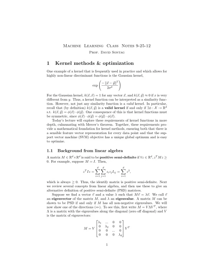
Machine Learning Class Notes 9-25-12 Prof. David Sontag 1 Kernel methods & optimization One example of a kernel that is frequently used in practice and which allows for highly non-linear discriminant functions is the Gaussian kernel, � � y � 2 − � � x − � exp 2 σ 2 For the Gaussian kernel, k ( � x, � x ) = 1 for any vector � x , and k ( � x, � y ) ≈ 0 if x is very different from y . Thus, a kernel function can be interpreted as a similarity func- tion. However, not just any similarity function is a valid kernel. In particular, y ) is a valid kernel if and only if ∃ φ : X → R d recall that (by definition) k ( � x, � s.t. k ( � x, � y ) = φ ( � x ) · φ ( � y ). One consequence of this is that kernel functions must be symmetric, since φ ( � x ) · φ ( � y ) = φ ( � y ) · φ ( � x ). Today’s lecture will explore these requirements of kernel functions in more depth, culmunating with Mercer’s theorem. Together, these requirements pro- vide a mathematical foundation for kernel methods, ensuring both that there is a sensible feature vector representation for every data point and that the sup- port vector machine (SVM) objective has a unique global optimum and is easy to optimize. 1.1 Background from linear algebra A matrix M ∈ R d × R d is said to be positive semi-definite if ∀ z ∈ R d , z T Mz ≥ 0. For example, suppose M = I . Then, d d d z T Iz = � � � z 2 , z i z j I ij = i =1 j =1 i =1 which is always ≥ 0. Thus, the identify matrix is positive semi-definite. Next we review several concepts from linear algebra, and then use these to give an alternative definition of positive semi-definite (PSD) matrices. Suppose we find a vector � v and a value λ such that M� v = λ� v . We call � v an eigenvector of the matrix M , and λ an eigenvalue . A matrix M can be shown to be PSD if and only if M has all non-negative eigenvalues. We will now show one of the directions ( ⇐ ). To see this, first write M = V Λ V T , where Λ is a matrix with the eigenvalues along the diagonal (zero off diagonal) and V is the matrix of eigenvectors: 0 0 λ 1 ... 0 0 0 λ 2 V T M = V 0 0 0 ... 0 0 0 λ d 1
Next, we split Λ in two, √ λ 1 √ λ 1 ... 0 0 ... 0 0 √ λ 2 √ λ 2 0 0 0 0 0 0 = UU T . V T M = V 0 0 ... 0 0 0 ... 0 √ λ d √ λ d 0 0 0 0 0 0 Letting v = z T U , since vv T = v · v ≥ 0 we have that ( z T U )( U T z ) = z T Mz ≥ 0, showing that M is positive semi-definite (we used the fact that the eigenvalues were non-negative when taking their square root). 1.2 Mercer’s Theorem For a training set S = { � x i } and a function k ( � u,� v ), the kernel matrix (also called the Gram matrix) K S is the matrix of dimension | S |×| S | where ( K S ) ij = k ( � x i , � x j ). Theorem 1 (Mercer’s theorem) . k ( � u,� v ) is a valid kernel if and only if the corresponding kernel matrix is PSD for all training sets S = { � x i } . Proof. ( ⇒ ) Since k ( � v ) is a valid kernel, it has a corresponding feature map u,� φ such that k ( � v ) = φ ( � u ) · φ ( � v ). Thus, the kernel matrix K s has entries u,� � φ ( x 1 ) φ ( x n ) � ( K S ) ij = φ ( � x i ) · φ ( � x j ). Let V be the matrix , where we ... treat φ ( x i ) as a column vector. Then, we have K S = V T V . However, thsi shows that K S must be positive semi-definite, because for any vector z ∈ R | S | , ( z T V T )( V z ) ≥ 0. ( ⇐ ) Let S be the set of all possible data points (we will assume that it is finite). Since the corresponding kernel matrix K S is positive semi-definite, it has non-negative eigenvalues and can be factored as K S = UU T . Let φ ( x i ) = u i , where u i is the i ’th row of U . This gives the feature mapping for x i such that k ( x i , x j ) = u i · u j . Mercer’s theorem guarantees for us that the kernel matrix is positive semi- definite. As we show in the next section, this will guarantee that the SVM dual objective is concave, which means that it is easy to optimize. 1.3 Convexity A set X ⊆ R d is a convex set if for any � x, � y ∈ X and 0 ≤ α ≤ 1, x + (1 − α ) � y ∈ X α� Informally, if for any two points � x , � y that are in the set every point on the line connecting � x and � y is also included in the set, then the set is convex. See Figure 1 for examples of non-convex and convex sets. A function f : X → R is convex for a convex set X if ∀ � x, � y ∈ X and 0 ≤ α ≤ 1, f ( α� x + (1 − α ) � y ) ≤ αf ( � x ) + (1 − α ) f ( � y ) (1) 2
Not convex: Convex: Set specified by linear inequalities: x ∈ R 2 : A� X = { � x ≤ b } Figure 1: Illustration of a non-convex and two convex sets in R 2 . Informally, a function is convex if the line between any two points on the curve always upper bounds the function. We call a function strictly convex if the inequality in Eq. 1 is a strict inequality. See See Figure 2 for examples of non- convex and convex functions. A function f ( x ) is concave is − f ( x ) is convex. Importantly, it can be shown that strictly convex functions always have a unique minima. For a function f ( x ) defined over the real line, one can show that f ( x ) is d 2 convex if and only if dx 2 f ≥ 0 ∀ x . Just as before, strict convexity occurs when the inequality is strict. For example, consider f ( x ) = x 2 . The first derivative of d 2 d f ( x ) is given by dx f = 2 x and its second derivative by dx 2 f = 2. Since this is always strictly greater than 0, we have proven that f ( x ) = x 2 is strictly convex. dx f = 1 d As a second example, consider f ( x ) = log( x ). The first derivative is x , d 2 dx 2 f = − 1 and its second derivative is given by x 2 . Since this is negative for all x > 0, we have proven that log( x ) is a concave function over R + . This matters because optimization for convex functions is easy. In partic- ular, one can show that nearly any reasonable optimization method, such as gradient descent (where one starts at arbitrary point, moves a little bit in the direction opposite to the gradient, and then repeats), is guaranteed to reach a global optimum of the function. Note that whereas the minimization of convex functions is easy, likewise, the maximization of concave functions is easy. Finally, to generalize this second definition of convex functions to higher dimensions (i.e., X = R d ), we introduce the notion of the Hessian matrix of Not convex: Convex: f ( x ) f ( x ) f ( x ) = x 2 x x x Figure 2: Illustration of a non-convex and two convex functions over X = R . 3
a function f , ∂ 2 f ∂ 2 f · · · ∂x 2 ∂x 1 ∂x d 1 . . ∇ 2 f ( � . . x ) = . . ∂ 2 f ∂ 2 f · · · ∂x d ∂x 1 ∂x 2 d which is the matrix of dimension d × d with entries ( ∇ 2 f ) ij equal to the partial derivative of the function with respect to x i and then with respect to x j , denoted ∂ 2 f ∂x i ∂x j . Note that since the order of the partial derivatives does not matter, i.e. ∂ 2 f ∂ 2 f ∂x i ∂x j = ∂x j ∂x i , the Hessian matrix is symmetric. We are finally ready for our second definition of convex functions in higher dimension. A function f : X → R is convex for a convex set X ⊆ R d if and only if its Hessian matrix ∇ 2 f ( � x ) is positive semi-definite for all � x ∈ X . 1.4 The dual SVM objective is concave Recall the dual of the support vector machine (SVM) objective, n n n α i − 1 � � � f ( � α ) = α i α j y i y j k ( x i , x j ) (2) 2 i =1 i =1 j =1 The first partial derivative is given by ∂f � = 1 − α i y i y s k ( x i , x s ) − α s k ( x s , x s ) ∂α s i � = s The second partial derivative is given by ∂ 2 f = − y t y s k ( x t , x s ) ∂α t ∂α s y ∈ {− 1 , 1 } n be the vector of assignments to the n data points (a column Let � y T K S � vector). We can then write the Hessian matrix ∇ 2 f as − � y , where K S is the kernel matrix for the n data points. Since k ( � v ) is a valid kernel, Mercer’s u,� theorem guarantees for us that K S is positive semi-definite. As a result, we z T K S � y T K� z ∈ R n . We conclude that − � have that � z ≥ 0 for all vectors � y ≤ 0, finishing our proof that the dual SVM objective is concave. There are many approaches for minimizing f ( � α ). One of the simplest such methods is called the sequential minimal optimization (SMO) algorithm, and is based on the concept of block coordinate descent . Coordinate descent is illustrated in Fig. 3 for a function defined on R 2 . An arbitrary starting point is chosen. Then, in each step, one coordinate (or, in general, a set of coordinates, called a block) is chosen and the function is minimized as much as possible with respect to that coordinate (keeping all other variables fixed to their current values). The larger the blocks, the faster the convergence to the optimum solution. The blocks are typically chosen to be as large as possible such that minimizing 4
Recommend
More recommend
Explore More Topics
Stay informed with curated content and fresh updates.
