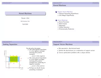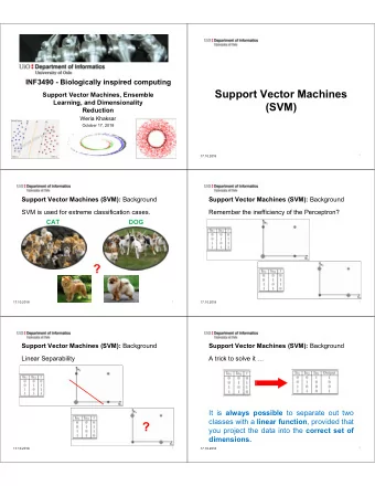
Support Vector Machines Preview What is a support vector machine? - PowerPoint PPT Presentation
Support Vector Machines Preview What is a support vector machine? The perceptron revisited Kernels Weight optimization Handling noisy data What Is a Support Vector Machine? 1. A subset of the training examples x (the support
Support Vector Machines
Preview • What is a support vector machine? • The perceptron revisited • Kernels • Weight optimization • Handling noisy data
What Is a Support Vector Machine? 1. A subset of the training examples x (the support vectors ) 2. A vector of weights for them α 3. A similarity function K ( x, x ′ ) (the kernel ) Class prediction for new example x q : �� � f ( x q ) = sign α i y i K ( x q , x i ) i ( y i ∈ {− 1 , 1 } )
• So SVMs are a form of instance-based learning • But they’re usually presented as a generalization of the perceptron • What’s the relation between perceptrons and IBL?
The Perceptron Revisited The perceptron is a special case of weighted kNN you get when the similarity function is the dot product : � f ( x q ) = sign w j x qj j But � w j = α i y i x ij i So �� � �� � � = sign f ( x q ) = sign α i y i x ij x qj α i y i ( x q · x i ) j i i
Another View of SVMs • Take the perceptron • Replace dot product with arbitrary similarity function • Now you have a much more powerful learner • Kernel matrix: K ( x, x ′ ) for x, x ′ ∈ Data • If a symmetric matrix K is positive semi-definite (i.e., has non-negative eigenvalues), then K ( x, x ′ ) is still a dot product, but in a transformed space: K ( x, x ′ ) = φ ( x ) · φ ( x ′ ) • Also guarantees convex weight optimization problem • Very general trick
Examples of Kernels Linear: K ( x, x ′ ) = x · x ′ Polynomial: K ( x, x ′ ) = ( x · x ′ ) d Gaussian: K ( x, x ′ ) = exp( − 1 2 � x − x ′ � /σ )
Example: Polynomial Kernel u = ( u 1 , u 2 ) v = ( v 1 , v 2 ) ( u · v ) 2 ( u 1 v 1 + u 2 v 2 ) 2 = u 2 1 v 2 1 + u 2 2 v 2 = 2 + 2 u 1 v 1 u 2 v 2 √ √ ( u 2 1 , u 2 2 u 1 u 2 ) · ( v 2 1 , v 2 = 2 , 2 , 2 v 1 v 2 ) = φ ( u ) · φ ( v ) • Linear kernel can’t represent quadratic frontiers • Polynomial kernel can
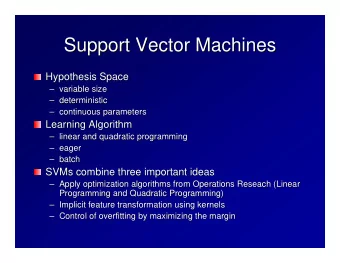
Learning SVMs So how do we: • Choose the kernel? Black art • Choose the examples? Side effect of choosing weights • Choose the weights? Maximize the margin
Maximizing the Margin
The Weight Optimization Problem • Margin = min y i ( w · x i ) • Easy to increase margin by increasing weights! • Instead: Fix margin, minimize weights • Minimize w · w y i ( w · x i ) ≥ 1, for all i Subject to
Constrained Optimization 101 • Minimize f ( w ) h i ( w ) = 0, for i = 1 , 2 , . . . Subject to • At solution w ∗ , ∇ f ( w ∗ ) must lie in subspace spanned by {∇ h i ( w ∗ ): i = 1 , 2 , . . . } • Lagrangian function: � L ( w, β ) = f ( w ) + β i h i ( w ) i • The β i s are the Lagrange multipliers • Solve ∇ L ( w ∗ , β ∗ ) = 0
Primal and Dual Problems • Problem over w is the primal • Solve equations for w and substitute • Resulting problem over β is the dual • If it’s easier, solve dual instead of primal • In SVMs: – Primal problem is over feature weights – Dual problem is over instance weights
Inequality Constraints • Minimize f ( w ) g i ( w ) ≤ 0, for i = 1 , 2 , . . . Subject to h i ( w ) = 0, for i = 1 , 2 , . . . • Lagrange multipliers for inequalities: α i • KKT Conditions: ∇ L ( w ∗ , α ∗ , β ∗ ) = 0 α ∗ ≥ 0 i g i ( w ∗ ) ≤ 0 α ∗ i g i ( w ∗ ) = 0 • Complementarity: Either a constraint is active ( g i ( w ∗ ) = 0) or its multiplier is zero ( α ∗ i = 0) • In SVMs: Active constraint ⇒ Support vector
Solution Techniques • Use generic quadratic programming solver • Use specialized optimization algorithm • E.g.: SMO (Sequential Minimal Optimization) – Simplest method: Update one α i at a time – But this violates constraints – Iterate until convergence: 1. Find example x i that violates KKT conditions 2. Select second example x j heuristically 3. Jointly optimize α i and α j
Handling Noisy Data
Handling Noisy Data • Introduce slack variables ξ i w · w + C � • Minimize i ξ i y i ( w · x i ) ≥ 1 − ξ i , for all i Subject to
Bounds Margin bound: Bound on VC dimension decreases with margin Leave-one-out bound: E [ error D ( h )] ≤ E [# support vectors] # examples
Support Vector Machines: Summary • What is a support vector machine? • The perceptron revisited • Kernels • Weight optimization • Handling noisy data
Recommend
More recommend
Explore More Topics
Stay informed with curated content and fresh updates.

