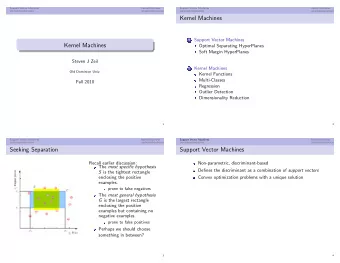
Support Vector Machines Support Vector Machines Hypothesis Space - PowerPoint PPT Presentation

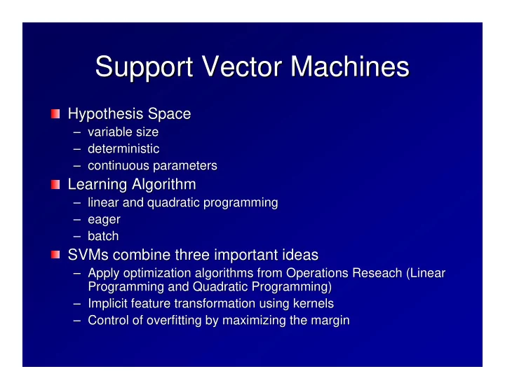
Support Vector Machines Support Vector Machines Hypothesis Space Hypothesis Space – variable size variable size – – deterministic deterministic – – continuous parameters continuous parameters – Learning Algorithm Learning Algorithm – linear and quadratic programming linear and quadratic programming – – eager – eager – batch batch – SVMs combine three important ideas SVMs combine three important ideas – Apply optimization algorithms from Operations Reseach (Linear Apply optimization algorithms from Operations Reseach (Linear – Programming and Quadratic Programming) Programming and Quadratic Programming) – Implicit feature transformation using kernels Implicit feature transformation using kernels – – Control of overfitting by maximizing the margin Control of overfitting by maximizing the margin –

White Lie Warning White Lie Warning This first introduction to SVMs describes a This first introduction to SVMs describes a special case with simplifying assumptions special case with simplifying assumptions We will revisit SVMs later in the quarter We will revisit SVMs later in the quarter and remove the assumptions and remove the assumptions The material you are about to see does The material you are about to see does not describe “ “real real” ” SVMs SVMs not describe

Linear Programming Linear Programming The linear programming problem is the The linear programming problem is the following: following: find w w find · w minimize c · w minimize c subject to subject to w · · a a i = b i for i i = 1, = 1, … …, , m m w i = b i for ≥ 0 for 0 for j j = 1, = 1, … …, , n w j j ≥ n w There are fast algorithms for solving linear There are fast algorithms for solving linear programs including the simplex algorithm and programs including the simplex algorithm and Karmarkar’ ’s algorithm s algorithm Karmarkar

Formulating LTU Learning as Formulating LTU Learning as Linear Programming Linear Programming Encode classes as {+1, – –1} 1} Encode classes as {+1, LTU: LTU: w · · x x ≥ ≥ 0 h(x) = +1 if w 0 h(x) = +1 if = – –1 otherwise 1 otherwise = An example ( x x i , y y i ) is classified correctly by h h if if An example ( i , i ) is classified correctly by · w w · · x > 0 y i i · x i i > 0 y Basic idea: The constraints on the linear Basic idea: The constraints on the linear programming problem will be of the form programming problem will be of the form · w w · · x y i i · x i > 0 y i > 0 We need to introduce two more steps to convert We need to introduce two more steps to convert this into the standard format for a linear program this into the standard format for a linear program

Converting to Standard LP Form Converting to Standard LP Form Step 1: Convert to equality constraints by using slack Step 1: Convert to equality constraints by using slack variables variables – Introduce one slack variable – Introduce one slack variable s s i i for each training example for each training example x x i i and and ≥ 0: require that s s i i ≥ 0: require that · w w · · x y i i · x i i – – s s i i = 0 = 0 y Step 2: Make all variables positive by subtracting pairs Step 2: Make all variables positive by subtracting pairs – Replace each Replace each w be a difference of two variables: w = u – v , – w j j be a difference of two variables: w j j = u j j – v j j , ≥ 0 where u where u j j , , v v j j ≥ 0 y i i · · ( ( u u – – v v ) ) · · x x i – s s i = 0 y i – i = 0 Linear program: Linear program: – Find Find s s i , u u j , v v j – i , j , j – Minimize (no objective function) Minimize (no objective function) – – Subject to: Subject to: – ∑ j ( ∑ y i i ( j ( ( u u j j – – v v j j ) ) x x ij ij ) ) – – s s i i = 0 = 0 y s i i ≥ ≥ 0, 0, u u j j ≥ ≥ 0, 0, v v j j ≥ ≥ 0 0 s The linear program will have a solution iff the points are The linear program will have a solution iff the points are linearly separable linearly separable

Example Example 30 random data points labeled according to the line x x 2 = 30 random data points labeled according to the line 2 = 1 + x x 1 1 + 1 Pink line is true classifier Pink line is true classifier Blue line is the linear programming fit Blue line is the linear programming fit

What Happens with What Happens with Non- -Separable Data? Separable Data? Non Bad News: Linear Program is Infeasible Bad News: Linear Program is Infeasible

Higher Dimensional Spaces Higher Dimensional Spaces Theorem: For any any data set, there exists a data set, there exists a Theorem: For Φ to a higher mapping Φ to a higher- -dimensional space dimensional space mapping such that the data is linearly separable such that the data is linearly separable Φ( ( X φ 1 φ 2 φ D Φ ) = ( φ ), φ , φ X ) = ( ( x x ), ( x x ), ), … …, ( x x )) )) 1 ( 2 ( D ( Example: Map to quadratic space Example: Map to quadratic space – x x = (x = (x 1 , x 2 ) (just two features) – 1 , x 2 ) (just two features) √ √ √ – Φ Φ ( ( x 2 2 x 1 x 2 , x 2 ( x ) = – x ) = 2 x 1 , 2 x 2 , 1) 1 , 2 , – compute linear separator in this space compute linear separator in this space –

Drawback of this approach Drawback of this approach The number of features increases rapidly The number of features increases rapidly This makes the linear program much This makes the linear program much slower to solve slower to solve

Kernel Trick Kernel Trick A dot product between two higher- - A dot product between two higher dimensional mappings can sometimes be dimensional mappings can sometimes be implemented by a kernel function kernel function implemented by a Φ ( · Φ Φ ( ) = Φ K( x x i , x x j ( x x i ) · ( x x j ) K( i , j ) = i ) j ) Example: Quadratic Kernel Example: Quadratic Kernel = ( x i · x j + 1) 2 K ( x i , x j ) = ( x i 1 x j 1 + x i 2 x j 2 + 1) 2 = x 2 i 1 x 2 j 1 + 2 x i 1 x i 2 x j 1 x j 2 + x 2 i 2 x 2 j 2 + 2 x i 1 x j 1 + 2 x i 2 x j 2 + 1 √ √ √ = ( x 2 2 x i 1 x i 2 , x 2 2 x i 1 , 2 x i 2 , 1) · i 1 , i 2 , √ √ √ ( x 2 2 x j 1 x j 2 , x 2 2 x j 1 , 2 x j 2 , 1) j 1 , j 2 , = Φ( x i ) · Φ( x j )

Idea Idea Reformulate the LTU linear program so Reformulate the LTU linear program so that it only involves dot products between that it only involves dot products between pairs of training examples pairs of training examples Then we can use kernels to compute Then we can use kernels to compute these dot products these dot products Running time of algorithm will not depend Running time of algorithm will not depend on number of dimensions D of high- - on number of dimensions D of high dimensional space dimensional space

Reformulating the Reformulating the LTU Linear Program LTU Linear Program Claim: In online Perceptron, w w can be written as can be written as Claim: In online Perceptron, ∑ j α j = ∑ j α w = j y y j x j w j x j Proof: Proof: – Each weight update has the form Each weight update has the form – η g + η w t := w w t g i,t w t := 1 + t- -1 i,t – g g i,t is computed as – i,t is computed as g i,t i,t = error = error it it y y i x i i (error (error it it = 1 if x = 1 if x i i misclassified in iteration t; 0 misclassified in iteration t; 0 g i x otherwise) otherwise) – Hence Hence – + ∑ ∑ t t ∑ ∑ i i η η error w t = w w 0 error it y i x i w t = 0 + it y i x i – But But w w 0 = (0, 0, … …, 0), so , 0), so – 0 = (0, 0, ∑ t ∑ i η error = ∑ t ∑ i η w t t = error it it y y i x i w i x i ∑ i ∑ t η error = ∑ ( ∑ t η w t t = i ( error it it ) y ) y i x i w i x i ∑ i α i = ∑ i α w t t = y i x i w i y i x i

Rewriting the Linear Separator Using Dot Products Rewriting the Linear Separator Using Dot Products ⎛ ⎞ ⎝ X ⎠ · x i = w · x i α j y j x j j X = α j y j ( x j · x i ) j Change of variables Change of variables α j , optimize { α – instead of optimizing instead of optimizing w w , optimize { }. – j }. – Rewrite the constraint Rewrite the constraint – w · · x > 0 as y i x i i > 0 as y i w ∑ j α j i ∑ j α · x ( x j · ) > 0 or y i y j j ( x j x i i ) > 0 or y j y ∑ j ∑ j α α j · x y j y i ( x x j j · x i ) > 0 j y j y i ( i ) > 0

The Linear Program becomes The Linear Program becomes α j Find { α – Find { } – j } – minimize (no objective function) minimize (no objective function) – – subject to subject to – ∑ j α j ∑ j α · x y j y i ( x x j j · x i ) > 0 j y j y i ( i ) > 0 α j α j ≥ ≥ 0 0 – Notes: Notes: – α j α j The weight α is. If α The weight j tells us how tells us how “ “important important” ” example example x x j j is. If j is is non- -zero, then zero, then x is called a “ “support vector support vector” ” non x j j is called a To classify a new data point x x , we take its dot product with , we take its dot product with To classify a new data point the support vectors the support vectors ∑ j α j ∑ j α · x y j ( x x j j · x ) > 0? ) > 0? j y j (