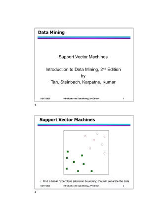
Support vector machines CS 446 Part 1: linear support vector - PowerPoint PPT Presentation

Support vector machines CS 446

Part 1: linear support vector machines 1.0 1.0 1.0 0.8 0.8 0.8 0 0 0 . 8 - 0.6 0.6 0.6 0 0 0 0 0 0 0 0 0 0 0 0 0 0 0 0 0 0 0 0 0 0 0 0 0 0 0 0 0 0 0 0 . 0 0 0 0 0 0 2 8 4 0 0 0 0 0 4 0 0 0 . 2 . 4 6 . . 0 0 . 0 4 8 2 . - . 0 0 8 . 0 . 8 6 1 . . 0 . 0 0 . 0 . 0 . . 1 6 2 . 0 2 . 3 2 1 - 1 - - - - - - - - 0.4 0.4 0.4 0 0 0 . 4 0.2 0.2 0.2 0.0 0.0 0.0 2.0 1.5 1.0 0.5 0.0 0.5 1.0 1.5 2.0 2.0 1.5 1.0 0.5 0.0 0.5 1.0 1.5 2.0 2.0 1.5 1.0 0.5 0.0 0.5 1.0 1.5 2.0 Logistic regression. Least squares. SVM. 1 / 39

Part 2: kernelized support vector machines 1.00 1.00 -12.500 0.75 0.75 -32.000 0.50 0.50 0 0 0 . -24.000 0 1 - -8.000 0.25 0.25 -7.500 0 0 0 -8.000 - 2 -2.500 0.00 6 . 0.00 -5.000 0.000 . 8.000 5 1 0 - 0 8.000 0 0 0 0 0 . 0 0 0 . 0 . 0 0 0 0.25 0.25 2 . 5 0 0 0.50 0.50 0.75 0.75 16.000 1.00 1.00 1.00 0.75 0.50 0.25 0.00 0.25 0.50 0.75 1.00 1.00 0.75 0.50 0.25 0.00 0.25 0.50 0.75 1.00 ReLU network. Quadratic SVM. 1.00 1.00 0.75 0.75 - 1 0 . 0.50 0.50 0 0 0 0 0 0.25 0.25 . 3 0.500 - -0.500 0 -1.000 -1.000 0 0 0.00 0 0.00 0.500 0 . 2 5 0 . - 0.000 1 1.000 0 - 0 1 0 -0.500 . . . 5 0 1 0 0.25 - 0.25 0 -1.000 0 0 0 0 0 0 0 . 0.50 0 2.000 0.50 0 . 0 0.75 0.75 0 1.00 1.00 0 3.000 0 . 1 1.00 0.75 0.50 0.25 0.00 0.25 0.50 0.75 1.00 1.00 0.75 0.50 0.25 0.00 0.25 0.50 0.75 1.00 RBF SVM. Narrower RBF SVM. 2 / 39

1. Recap: linearly separable data

Linear classifiers (with Y = {− 1 , +1 } ) Linear separability assumption Assume there is a linear classifier that perfectly classifies the training data S : for some w ⋆ ∈ R d , T w ⋆ > 0 . ( x ,y ) ∈ S y x min 3 / 39

Linear classifiers (with Y = {− 1 , +1 } ) Linear separability assumption Assume there is a linear classifier that perfectly classifies the training data S : for some w ⋆ ∈ R d , T w ⋆ > 0 . ( x ,y ) ∈ S y x min Convex program Finding any such w is a convex (linear!) feasibility problem. 3 / 39

Linear classifiers (with Y = {− 1 , +1 } ) Linear separability assumption Assume there is a linear classifier that perfectly classifies the training data S : for some w ⋆ ∈ R d , T w ⋆ > 0 . ( x ,y ) ∈ S y x min Convex program Finding any such w is a convex (linear!) feasibility problem. Logistic regression Alternatively, can run enough steps of logistic regression. 3 / 39

Support vector machines (SVMs) Motivation ◮ Let’s first define a good linear separator, and then solve for it. ◮ Let’s also find a principled approach to nonseparable data. 4 / 39

Support vector machines (SVMs) Motivation ◮ Let’s first define a good linear separator, and then solve for it. ◮ Let’s also find a principled approach to nonseparable data. Support vector machines (Vapnik and Chervonenkis, 1963) ◮ Characterize a stable solution for linearly separable problems—the maximum margin solution . ◮ Solve for the maximum margin solution efficiently via convex optimization. ◮ Convex dual has valuable structure; it will give useful extensions, and is what we’ll optimize. ◮ Extend the optimization problem to non-separable data via convex surrogate losses . ◮ Nonlinear separators via kernels . 4 / 39

2. Maximum margin solution

Maximum margin solution Best linear classifier on population 5 / 39

Maximum margin solution Best linear classifier on Arbitrary linear separator on population training data S 5 / 39

Maximum margin solution Best linear classifier on Arbitrary linear separator on population training data S 5 / 39

Maximum margin solution Best linear classifier on Arbitrary linear separator on Maximum margin solution on population training data S training data S 5 / 39

Maximum margin solution Best linear classifier on Arbitrary linear separator on Maximum margin solution on population training data S training data S 5 / 39

Maximum margin solution Best linear classifier on Arbitrary linear separator on Maximum margin solution on population training data S training data S Why use the maximum margin solution ? (i) Uniquely determined by S , unlike the linear program. (ii) It is a particular inductive bias—i.e., an assumption about the problem—that seems to be commonly useful. ◮ We’ve seen inductive bias: least squares and logistic regression choose different predictors on same data. ◮ This particular bias (margin maximization) is common in machine learning, has many nice properties. 5 / 39

Maximum margin solution Best linear classifier on Arbitrary linear separator on Maximum margin solution on population training data S training data S Why use the maximum margin solution ? (i) Uniquely determined by S , unlike the linear program. (ii) It is a particular inductive bias—i.e., an assumption about the problem—that seems to be commonly useful. ◮ We’ve seen inductive bias: least squares and logistic regression choose different predictors on same data. ◮ This particular bias (margin maximization) is common in machine learning, has many nice properties. Key insight : can express this as another convex program. 5 / 39

Distance to decision boundary Suppose w ∈ R d satisfies T w > 0 . ( x ,y ) ∈ S y x min 6 / 39

Distance to decision boundary Suppose w ∈ R d satisfies T w > 0 . ( x ,y ) ∈ S y x min ◮ “Maximum margin” shouldn’t care about scaling; w and 10 w should be equally good. ◮ Thus for each direction w / � w � , we can fix a scaling. 6 / 39

Distance to decision boundary Suppose w ∈ R d satisfies T w > 0 . ( x ,y ) ∈ S y x min ◮ “Maximum margin” shouldn’t care about scaling; w and 10 w should be equally good. ◮ Thus for each direction w / � w � , we can fix a scaling. Let (˜ x , ˜ y ) be any example in S that achieves the minimum. 6 / 39

Distance to decision boundary Suppose w ∈ R d satisfies T w > 0 . ( x ,y ) ∈ S y x min ◮ “Maximum margin” shouldn’t care about scaling; w and 10 w should be equally good. ◮ Thus for each direction w / � w � , we can fix a scaling. Let (˜ x , ˜ y ) be any example in S that achieves the minimum. H x T w ˜ y ˜ y ˜ ˜ x � w � 2 w 6 / 39

Distance to decision boundary Suppose w ∈ R d satisfies T w > 0 . ( x ,y ) ∈ S y x min ◮ “Maximum margin” shouldn’t care about scaling; w and 10 w should be equally good. ◮ Thus for each direction w / � w � , we can fix a scaling. Let (˜ x , ˜ y ) be any example in S that achieves the minimum. ◮ Rescale w so that ˜ y ˜ x T w = 1 . (Now scaling is fixed.) H x T w ˜ y ˜ y ˜ ˜ x � w � 2 w 6 / 39

Distance to decision boundary Suppose w ∈ R d satisfies T w > 0 . ( x ,y ) ∈ S y x min ◮ “Maximum margin” shouldn’t care about scaling; w and 10 w should be equally good. ◮ Thus for each direction w / � w � , we can fix a scaling. Let (˜ x , ˜ y ) be any example in S that achieves the minimum. ◮ Rescale w so that ˜ y ˜ x T w = 1 . (Now scaling is fixed.) H x T w ˜ y ˜ y ˜ ˜ 1 x � w � 2 ◮ Distance from ˜ y ˜ x to H is . � w � 2 This is the (normalized minimum) margin. w 6 / 39

Distance to decision boundary Suppose w ∈ R d satisfies T w > 0 . ( x ,y ) ∈ S y x min ◮ “Maximum margin” shouldn’t care about scaling; w and 10 w should be equally good. ◮ Thus for each direction w / � w � , we can fix a scaling. Let (˜ x , ˜ y ) be any example in S that achieves the minimum. ◮ Rescale w so that ˜ y ˜ x T w = 1 . (Now scaling is fixed.) H x T w ˜ y ˜ y ˜ ˜ 1 x � w � 2 ◮ Distance from ˜ y ˜ x to H is . � w � 2 This is the (normalized minimum) margin. w ◮ This gives optimization problem max 1 / � w � T w = 1 . subj. to ( x ,y ) ∈ S y x min Can make constraint ≥ 1 . 6 / 39

Maximum margin linear classifier The solution ˆ w to the following mathematical optimization problem: 1 2 � w � 2 min 2 w ∈ R d T w ≥ 1 s.t. y x for all ( x , y ) ∈ S gives the linear classifier with the largest minimum margin on S —i.e., the maximum margin linear classifier or support vector machine (SVM) classifier . 7 / 39

Maximum margin linear classifier The solution ˆ w to the following mathematical optimization problem: 1 2 � w � 2 min 2 w ∈ R d T w ≥ 1 s.t. y x for all ( x , y ) ∈ S gives the linear classifier with the largest minimum margin on S —i.e., the maximum margin linear classifier or support vector machine (SVM) classifier . This is a convex optimization problem ; can be solved in polynomial time. 7 / 39

Maximum margin linear classifier The solution ˆ w to the following mathematical optimization problem: 1 2 � w � 2 min 2 w ∈ R d T w ≥ 1 s.t. y x for all ( x , y ) ∈ S gives the linear classifier with the largest minimum margin on S —i.e., the maximum margin linear classifier or support vector machine (SVM) classifier . This is a convex optimization problem ; can be solved in polynomial time. If there is a solution (i.e., S is linearly separable), then the solution is unique . 7 / 39