Linear Programming Outline Introduction Introduction A diet - PowerPoint PPT Presentation
Linear Programming Outline Introduction Introduction A diet problem A diet problem History of linear programming History of linear programming Applications Applications The Network Flow Problems The
Linear Programming
Outline Introduction Introduction A diet problem A diet problem History of linear programming History of linear programming Applications Applications The Network Flow Problems The Network Flow Problems Network Algorithms Network Algorithms Outline of Integer Programming Outline of Integer Programming
Introduction A Diet Problem A Diet Problem eg eg: Polly wonders how much money she must spend on food in order to get all the : Polly wonders how much money she must spend on food in order to get all the energy (2,000 kcal ), protein (50 g), and calcium (800 mg) that she needs every day. energy (2,000 kcal ), protein (50 g), and calcium (800 mg) that she needs every day. She choose six foods that seem to be cheap sources of the nutrients: She choose six foods that seem to be cheap sources of the nutrients: Food Serving Energy Protein (g) Calcium Price per size (kcal) (mg) serving (c) Oatmeal 28 g 110 4 2 3 Chicken 100 g 205 32 12 24 Eggs 2 large 160 13 54 13 Whole Milk 237 cc 160 8 285 9 Cherry pie 170 g 420 4 22 20 Pork with 260 g 260 14 80 19 beans
Introduction Servings-per-day limits on all six foods: Servings-per-day limits on all six foods: Oatmeal at most 4 servings per day Oatmeal at most 4 servings per day Chicken at most 3 servings per day Chicken at most 3 servings per day Eggs Eggs at most 2 servings per day at most 2 servings per day Milk at most 8 servings per day Milk at most 8 servings per day Cherry pie at most 2 servings per day Cherry pie at most 2 servings per day Pork with beans at most 2 servings per day at most 2 servings per day Pork with beans Now there are so many combinations seem promising that one could go on Now there are so many combinations seem promising that one could go on and on, looking for the best one. Trial and error is not particularly helpful and on, looking for the best one. Trial and error is not particularly helpful here. here.
Introduction A new way to express this— —using inequalities: using inequalities: A new way to express this minimize 3 x 24 x 13 x 9 x 20 x 19 x + + + + + 1 2 3 4 5 6 0 x 4 ! ! 1 subject to 0 x 3 ! ! 2 x 0 2 ! ! 3 0 x 8 ! ! 4 0 x 2 ! ! 5 0 x 2 ! ! 6 110 x 205 x 160 x 160 x 420 x 260 x 1 , 000 + + + + + ! 1 2 3 4 5 6 4 x 32 x 13 x 8 x 4 x 14 x 55 + + + + + ! 1 2 3 4 5 6 2 x 12 x 54 x 285 x 22 x 80 x 800 + + + + + ! 1 2 3 4 5 6
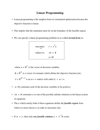
Introduction Problems of this kind are called “ “linear programming problems linear programming problems” ” or or “ “LP problems LP problems” ” for for Problems of this kind are called short; linear programming is the branch of applied mathematics concerned with short; linear programming is the branch of applied mathematics concerned with these problems. these problems. A A linear programming problem linear programming problem is the problem of maximizing (or minimizing) a linear is the problem of maximizing (or minimizing) a linear function subject to a finite number of linear constraints. function subject to a finite number of linear constraints. Standard form: Standard form: n c j x ! j maximize j 1 = n a x b ( i 1 , 2 , ..., m ) # " = ij j i subject to j 1 = x 0 ( j 1 , 2 , ..., n ) ! = j
History of Linear Programming It started in 1947 when It started in 1947 when G.B.Dantzig G.B.Dantzig design the design the “simplex method simplex method” ” for solving linear programming for solving linear programming “ formulations of U.S. Air Force planning formulations of U.S. Air Force planning problems. problems. It soon became clear that a surprisingly wide It soon became clear that a surprisingly wide range of apparently unrelated problems in range of apparently unrelated problems in production management could be stated in production management could be stated in linear programming terms and solved by the linear programming terms and solved by the simplex method. simplex method. Later, it was used to solve problems of Later, it was used to solve problems of management. It ʼ ʼ s algorithm can also used to s algorithm can also used to management. It network flow problems. network flow problems.
History of Linear Programming On Oct.14th,1975, the Royal Sweden Academy of Science awarded the Nobel On Oct.14th,1975, the Royal Sweden Academy of Science awarded the Nobel Prize in economic science to L.V.Kantorovich L.V.Kantorovich and and T.C.Koopmans T.C.Koopmans ” ”for their for their Prize in economic science to contributions to the theory of optimum allocation of resources contributions to the theory of optimum allocation of resources” ” The breakthrough in looking for a theoretically satisfactory algorithm to solve LP The breakthrough in looking for a theoretically satisfactory algorithm to solve LP problems came in 1979 when problems came in 1979 when L.G.Khachian L.G.Khachian published a description of such an published a description of such an algorithm. algorithm.
Applications Efficient allocation of scarce resources Efficient allocation of scarce resources diet problem diet problem Scheduling production and inventory Scheduling production and inventory multistage scheduling problems multistage scheduling problems The cutting-stock problem The cutting-stock problem find a way to cut paper or textiles rolls by find a way to cut paper or textiles rolls by complicated summary of orders complicated summary of orders Approximating data by linear functions Approximating data by linear functions find approximate solutions to possibly find approximate solutions to possibly unsolvable systems of linear equations unsolvable systems of linear equations
The Network Flow Problems The network flow problem concerns The network flow problem concerns finding the cheapest way to ship finding the cheapest way to ship 1 5 prescribed amounts of a commodity prescribed amounts of a commodity such as oranges from specified origins such as oranges from specified origins to specified destinations through a to specified destinations through a concrete transportation network concrete transportation network 4 Nodes Nodes Sinks Sinks Sources Sources 3 intermediate intermediate arcs: an order pair (i, j) of distinct arcs: an order pair (i, j) of distinct nodes i and j nodes i and j 2 Assumption: The total supply equals Assumption: The total supply equals 6 the total demand the total demand 7
The Network Flow Problems It is convenient to write each It is convenient to write each positive next to the positive next to the x 1 ij corresponding arc ij ij and to and to corresponding arc completely ignore arcs ij completely ignore arcs ij with = with = 0 0 x 2 2 ij x ij 6 Some requirements Some requirements 3 9 4 10 2 4
The Network Flow Problems x Ax = b, x >= 0 & # Ax = b, x >= 0 13 $ ! x 14 $ ! with x $ ! 15 $ ! x $ ! 21 1 1 1 1 1 $ x ! 0 ' ' ' & # & # 23 $ ! $ ! $ ! 1 1 1 1 1 1 x 0 ' ' ' ' $ ! $ ! 24 $ ! 1 1 1 $ ! $ ! 6 x $ ! 25 $ ! x $ ! = $ ! A 1 1 1 = b 10 = x $ ! $ ! $ ! 54 $ 1 1 1 1 ! ' 8 $ ! $ ! x $ ! 61 $ ! $ ! 1 1 1 1 ' ' ' ' 9 $ ! ' x $ ! $ ! 62 $ ! 1 1 1 ' ' $ ! 15 % " $ ! ' % " x $ ! 63 x $ ! 67 $ ! x $ ! 72 $ ! x % " 75
The Network Flow Problems Matrix A is called the incidence matrix of our network Matrix A is called the incidence matrix of our network Each component of the demand vector b specifies the demand at node i, with supplies Each component of the demand vector b specifies the demand at node i, with supplies b interpreted as negative demands interpreted as negative demands i Denote the cost of shipping a unit amount along Denote the cost of shipping a unit amount along ij ij by by c ij [ ] c c c c c c c c c c c c c c c = 13 14 15 21 23 24 25 54 61 62 63 67 72 75 [ ] 53 18 29 8 60 28 37 5 44 38 98 14 23 59 = Now the total cost of a schedule x equals Now the total cost of a schedule x equals cx c ij x ! = ij
The Network Flow Problems So the network flow problems is any problem: So the network flow problems is any problem: cx Ax b , x 0 minimize subject to = ! such that A is the n × m incidence matrix of some network and such that such that A is the n × m incidence matrix of some network and such that n b 0 ! = i this requirement stipulates assumption: The total supply equals the total demand this requirement stipulates assumption: The total supply equals the total demand i 1 =
Recommend
More recommend
Explore More Topics
Stay informed with curated content and fresh updates.
