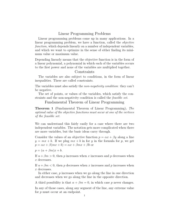
Linear Programming Problems Linear programming problems come up in - PDF document

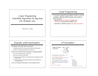
Linear Programming Problems Linear programming problems come up in many applications. In a linear programming problem, we have a function, called the objective function , which depends linearly on a number of independent variables, and which we want to optimize in the sense of either finding its mini- mum value or maximum value. Depending linearly means that the objective function is in the form of a linear polynomial, a polynomial in which each of the variables occurs to the first power and none of the variables are multiplied together. Constraints The variables are also subject to conditions, in the form of linear inequalities. These are called constraints. The variables must also satisfy the non-negativity condition : they can’t be negative. The set of points, or values of the variables, which satisfy the con- straints and the non-negativity condition is called the feasible set . Fundamental Theorem of Linear Programming Theorem 1 (Fundamental Theorem of Linear Programming) . The optimal value of the objective functions must occur at one of the vertices of the feasible set. We can understand this fairly easily for a case where there are two independent variables. The notation gets more complicated when there are more variables, but the basic ideas carry through. Consider the values of an objective function p = αx + βy along a line y = mx + b . If we plug mx + b in for y in the formula for p , we get p = αx + β ( mx + b ) = αx + βmx + βb or p = ( α + βm ) x + b . If α + βm > 0, then p increases when x increases and p decreases when x decreases. If α + βm < 0, then p decreases when x increases and p increases when x decreases. In either case, p increases when we go along the line in one direction and decreases when we go along the line in the opposite direction. A third possibility is that α + βm = 0, in which case p never changes. In any of those cases, along any segment of the line, any extreme value for p must occur at an endpoint. 1

2 If an extreme value occurs in a closed polygon, we easily see the ex- treme value must occur along the boundary, and then if it occurs along the boundary it must occur at one of the vertices, which is what the Fundamental Theorem of Linear Programming says. In a linear programming problem with just two variables and a hand- ful of constraints, it’s easy to sketch the feasible set and find its vertices. This is the essence of solving linear programming problems geometri- cally. • Find the feasible set. • Find the vertices. • Evaluate the objective function at each vertex. • Pick out the optimal value for the objective function. We’ll do some examples to help understand linear programming problems, but most linear programming problems that come up in real life involve numerous variables and constraints and effectively require a more efficient approach. The most common approach is called the Simplex Method . The Elephant in the Room Linear programming problems don’t come out of thin air; there are real problems that, when translated, turn into linear programming problems. The process of turning a real problem into a linear programming prob- lem is the same involved in any other word problem: Read the prob- lem!!! In particular, • Look for variables and unknowns. • Find connections among the variables and unknowns. In this case, the connections translate into constraints along with the objective function. The Simplex Method In most word problems studied before, the connections translated to equations, which were then solved. In linear programming problems, we generally use the Simplex Method . An Example Consider the following maximum problem:

3 2 x + y ≤ 3 3 x + y ≤ 4 x ≥ 0 , y ≥ 0 p = 17 x + 5 y Vertices The vertices of the feasible set and the values of the objective func- tion p = 17 x + 5 y at those points are the following: (0 , 0) 0 22 2 (4 / 3 , 0) 3 . (1 , 1) 22 (0 , 3) 15 Thus, the maximum value for p is 22 2 3 , which occurs at (4 / 3 , 0). The Simplex Method With the Simplex Method, we do not need to evaluate the objective function at each vertex. We will illustrate the Simplex Method using this example and then generalize the method so we can perform it mechanically, as an algo- rithm. The first step is to change the contraints from inequalities into equa- tions by introducing what are called slack variables . The slack variables essentially take up the slack in the inequalities. Looking at the inequality 2 x + y ≤ 3, we introduce the slack variable u = 3 − (2 x + y ), so u ≥ 0 while 2 x + y + u = 3. Similarly, looking at the inequality 3 x + y ≤ 4, we introduce the slack variable v = 4 − (3 x + y ), so v ≥ 0 while 3 x + y + v = 4. Restating the Problem We can thus restate the problem as 2 x + y + u = 3 3 x + y + v = 4 x, y, u, v ≥ 0 p = 17 x + 5 y where we find the maximum value for the objective function p which satisfies the contraints, now given as equations, and the non-negativity condition. A New System of Equations

4 If we rewrite the formula for the objective function in the form − 17 x − 5 y + p = 0, we get a system of equations: 2 x + y + u = 3 3 x + y + v = 4 − 17 x − 5 y + p = 0 . We will write down the augmented matrix for this system, use it to easily pick out one of the vertices and the value of the objective function at that vertex, and then pivot in a way that will enable us to find another vertex at which the value for the objective function is larger. The Initial Simplex Tableau The augmented matrix for the system 2 x + y + u = 3 3 x + y + v = 4 − 17 x − 5 y + p = 0 . is   x y u v p 2 1 1 0 0 3     3 1 0 1 0 4   − 17 − 5 0 0 1 0 The first row isn’t actually part of the augmented matrix, but we’ll write it down as a reminder of which variable each column is associated with. The Initial Tableau   x y u v p 2 1 1 0 0 3     3 1 0 1 0 4   − 17 − 5 0 0 1 0 Looking at the matrix, it’s fairly obvious that the columns corre- sponding to x and y are the most complicated. We can easily read off a solution if we set x = 0 and y = 0. If we do that, the first row, which corresponds to the equation 2 x + y + u = 3, gives a solution u = 3. Similarly, the second row, which corresponds to the equation 3 x + y + v = 4, gives a solution v = 4. The third row, which corresponds to the equation − 17 x − 5 y + p = 0, gives a solution p = 0. A Solution

5 So we have a solution of the equations giving x = 0, y = 0, u = 3, v = 4 and p = 0. This corresponds to the vertex (0 , 0), which gives a value of 0 for the objective function. We will call x and y Group I variables and we will call u and v Group II variables. Each time we pivot, we will exchange one pair of variables, one from Group I and one from Group II, to get another set of Group I variables which will be set to 0. This will give another fairly obvious solution, which will correspond to another vertex and another value of the ob- jective function. The Objective Function The last row gives a formula − 17 x − 5 y + p = 0 involving the objective function. We can solve this for the objective function, getting p = 17 x + 5 y . It may seem as if we’re going around in circles, but right now we’re trying to understand a process; later we will synthesize the ideas into an efficient algorithm. Since at the solution we found, x = y = 0, p takes on the value 0. On the other hand, it’s clear that if we found another solution where either x or y was positive, we’d get a larger value for p . It should also be clear that increasing x will increase p faster than increasing y would, so we’ll pivot in a way that will make x a Group II variable. We’ll do this by pivoting about the column corresponding to x , in other words, we’ll pivot about the first column. Finding the Pivot Row We now have to decide which entry in the first column to pivot around. Since the last row corresponds to the objective function, which is different in character from the others, we won’t even consider pivoting about the last row. If we pivoted about the first row, we’d start by dividing the first row by 2, getting 3 / 2 in the last column. We’d next subtract 3 times the first row from the second, which would give − 1 2 in the last column. Since negative numbers are evil, we’ll avoid that by pivoting about the second row. So we’ll pivot about the entry in the second row, first column. The Pivot   2 1 1 0 0 3 3 1 0 1 0 4   − 17 − 5 0 0 1 0 First, we divide the second row by 3 to get a 1 at the pivot point: