Introduction to Linear Programming Linear Programming is the study of - PowerPoint PPT Presentation

Introduction to Linear Programming

Linear Programming is the study of optimization problems in which the objective function and all constraints are linear.

Linear Programming is the study of optimization problems in which the objective function and all constraints are linear. A linear function in n variables is one of the form f ( x 1 , x 2 , . . . , x n ) = c 1 x 1 + c 2 x 2 + · · · + c n x n for some constants c 1 , c 2 , . . . , c n .

Linear Programming is the study of optimization problems in which the objective function and all constraints are linear. A linear function in n variables is one of the form f ( x 1 , x 2 , . . . , x n ) = c 1 x 1 + c 2 x 2 + · · · + c n x n for some constants c 1 , c 2 , . . . , c n . A linear inequality in n variables if one of the form f ( x 1 , x 2 , . . . , x n ) ≤ b or f ( x 1 , x 2 , . . . , x n ) ≥ b where f is a linear function and b is a constant.

Linear Programming is the study of optimization problems in which the objective function and all constraints are linear. A linear function in n variables is one of the form f ( x 1 , x 2 , . . . , x n ) = c 1 x 1 + c 2 x 2 + · · · + c n x n for some constants c 1 , c 2 , . . . , c n . A linear inequality in n variables if one of the form f ( x 1 , x 2 , . . . , x n ) ≤ b or f ( x 1 , x 2 , . . . , x n ) ≥ b where f is a linear function and b is a constant. Linear Programming is concerned with optimizing a linear function subject to a set of constraints given by linear inequalities.

A linear program (an LP ) is a linear optimization problem taking the following form: Maximize (or minimize) f ( x 1 , x 2 , . . . , x n ) = c 1 x 1 + c 2 x 2 + · · · + c n x n subject to ≤ a 1 , 1 x 1 + a 1 , 2 x 2 + · · · a 1 , n x n ≥ b 1 ≤ a 2 , 1 x 1 + a 2 , 2 x 2 + · · · a 2 , n x n ≥ b 2 : : ≤ a m , 1 x 1 + a m , 2 x 2 + · · · a m , n x n ≥ b m x 1 , x 2 , . . . x n ≥ 0 The inequalities, except for the last one, can be greater than or equal or less than or equal.

This general form is often expressed with vectors and matrices:

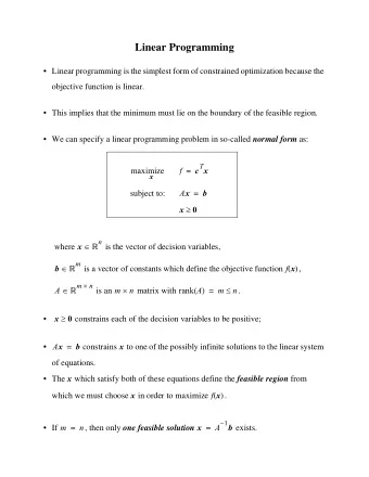
This general form is often expressed with vectors and matrices: Maximize (or minimize) c T � x x ≤ � subject to A � b ≥ and � x ≥ 0

This general form is often expressed with vectors and matrices: Maximize (or minimize) c T � x x ≤ � subject to A � b ≥ and � x ≥ 0 This looks very concise but it obscures a lot of things we will want to talk about, so I will not use this form at all. You will run across it in some papers and books on the subject.

LP example Suppose we are making salsa and guacamole (dips or sauces originally from Mexico).

LP example Suppose we are making salsa and guacamole (dips or sauces originally from Mexico). One unit of salsa requires 5 tomatoes and 1 clove of garlic.

LP example Suppose we are making salsa and guacamole (dips or sauces originally from Mexico). One unit of salsa requires 5 tomatoes and 1 clove of garlic. One unit of guacamole requires 1 / 2 tomato and 4 cloves of garlic.

LP example Suppose we are making salsa and guacamole (dips or sauces originally from Mexico). One unit of salsa requires 5 tomatoes and 1 clove of garlic. One unit of guacamole requires 1 / 2 tomato and 4 cloves of garlic. We only have 30 tomatoes and 20 cloves of garlic.

LP example Suppose we are making salsa and guacamole (dips or sauces originally from Mexico). One unit of salsa requires 5 tomatoes and 1 clove of garlic. One unit of guacamole requires 1 / 2 tomato and 4 cloves of garlic. We only have 30 tomatoes and 20 cloves of garlic. We have an unlimited supply of all other ingredients (salt, cilantro, lime juice, etc.)

LP example Suppose we are making salsa and guacamole (dips or sauces originally from Mexico). One unit of salsa requires 5 tomatoes and 1 clove of garlic. One unit of guacamole requires 1 / 2 tomato and 4 cloves of garlic. We only have 30 tomatoes and 20 cloves of garlic. We have an unlimited supply of all other ingredients (salt, cilantro, lime juice, etc.) How many units of salsa and guacamole should we make to maximize the total number of units (salsa+guacamole) we make?

LP example Suppose we are making salsa and guacamole (dips or sauces originally from Mexico). One unit of salsa requires 5 tomatoes and 1 clove of garlic. One unit of guacamole requires 1 / 2 tomato and 4 cloves of garlic. We only have 30 tomatoes and 20 cloves of garlic. We have an unlimited supply of all other ingredients (salt, cilantro, lime juice, etc.) How many units of salsa and guacamole should we make to maximize the total number of units (salsa+guacamole) we make? Fractional units are okay.

Let x 1 be the number of units of salsa we make. Let x 2 be the number of units of guacamole we make.

Let x 1 be the number of units of salsa we make. Let x 2 be the number of units of guacamole we make. Then the quantity we want to maximize is x 1 + x 2 . This is our objective function .

Let x 1 be the number of units of salsa we make. Let x 2 be the number of units of guacamole we make. Then the quantity we want to maximize is x 1 + x 2 . This is our objective function . We see that we cannot simply make x 1 and x 2 huge due to our limited amount of garlic and tomatoes.

If we make x 1 units of salsa and x 2 units of guacamole, then the amount of tomatoes we’ll need is 5 x 1 + 1 2 x 2 .

If we make x 1 units of salsa and x 2 units of guacamole, then the amount of tomatoes we’ll need is 5 x 1 + 1 2 x 2 . Since we only have 30 tomatoes, we have the following constraint 5 x 1 + 1 2 x 2 ≤ 30 .

If we make x 1 units of salsa and x 2 units of guacamole, then the amount of tomatoes we’ll need is 5 x 1 + 1 2 x 2 . Since we only have 30 tomatoes, we have the following constraint 5 x 1 + 1 2 x 2 ≤ 30 . Similarly, since we have a limited amount of garlic, we have another constraint : x 1 + 4 x 2 ≤ 20 .

If we make x 1 units of salsa and x 2 units of guacamole, then the amount of tomatoes we’ll need is 5 x 1 + 1 2 x 2 . Since we only have 30 tomatoes, we have the following constraint 5 x 1 + 1 2 x 2 ≤ 30 . Similarly, since we have a limited amount of garlic, we have another constraint : x 1 + 4 x 2 ≤ 20 . We also require x 1 , x 2 ≥ 0 since we cannot make a negative amount of salsa or guacamole.

Thus, the LP we wish to solve is: Maximize x 1 + x 2 subject to: 5 x 1 + 1 2 x 2 ≤ 30 x 1 + 4 x 2 ≤ 20 x 1 , x 2 ≥ 0 Since the non-negative constraints are always with us, we will often refer to such an LP as having two variables and two constraints.

In this course, we will not be concerned with the methods used or solving LPs.

In this course, we will not be concerned with the methods used or solving LPs. Instead, we will focus on lots of different applications of the LP idea, and we will use software to solve the LPs for us. In Math 407, you will learn methods for solving LPs.

Just once, though, let’s look at how we might solve our salsa and guacamole LP “by hand”.

Just once, though, let’s look at how we might solve our salsa and guacamole LP “by hand”. A classic approach (for two-variable LPs) is to consider the LP graphically.

Just once, though, let’s look at how we might solve our salsa and guacamole LP “by hand”. A classic approach (for two-variable LPs) is to consider the LP graphically. We begin by making a sketch of our inequalities.

The feasible region is the set of points ( x 1 , x 2 ) that satisfy both constraints. This is the doubly-shaded portion in the picture.

The feasible region is the set of points ( x 1 , x 2 ) that satisfy both constraints. This is the doubly-shaded portion in the picture. The points in the feasible region represent combinations of amounts of salsa and quacamole that we can make.

The feasible region is the set of points ( x 1 , x 2 ) that satisfy both constraints. This is the doubly-shaded portion in the picture. The points in the feasible region represent combinations of amounts of salsa and quacamole that we can make. Other points are not feasible.

We note that our objective function x 1 + x 2 is an increasing function of x 1 and x 2 .

We note that our objective function x 1 + x 2 is an increasing function of x 1 and x 2 . This means that, if ( x 1 , x 2 ) is a point in the feasible region, it will not yield the maximum value of x 1 + x 2 unless the point is “pushed up” against one of the constraint lines.

We note that our objective function x 1 + x 2 is an increasing function of x 1 and x 2 . This means that, if ( x 1 , x 2 ) is a point in the feasible region, it will not yield the maximum value of x 1 + x 2 unless the point is “pushed up” against one of the constraint lines. That is, if ( x 1 , x 2 ) is in the feasible region, and not on one of the constraint lines, then we can increase the value of x 1 + x 2 by increasing x 1 or x 2 . Hence, that point does not yield the maximum.