Linear Programming Linear programming is the simplest form of - PDF document

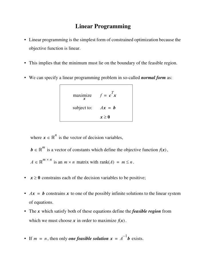
Linear Programming • Linear programming is the simplest form of constrained optimization because the objective function is linear. • This implies that the minimum must lie on the boundary of the feasible region. • We can specify a linear programming problem in so-called normal form as: c T x maximize f = x subject to: A x = b ≥ x 0 R n ∈ where x is the vector of decision variables, R m ∈ b is a vector of constants which define the objective function f x ( ), × R m n ∈ × ≤ A is an m n matrix with rank A ( ) = m n . ≥ • x constrains each of the decision variables to be positive; 0 • A x = b constrains x to one of the possibly infinite solutions to the linear system of equations. • The x which satisfy both of these equations define the feasible region from which we must choose x in order to maximize f x ( ). – b A 1 • If m = , then only one feasible solution x = exists. n

• If one also has inequality constraints given by T x ≤ a i b i then one can introduce “ slack variables ” such that: T x a i + x n = b i + 1 ≥ x n 0 + 1 T This will add one more row to the matrix A , that is a i one more element b to the vector b , and one more decision variable x n + to the vector of decision variables x . 1 • In this way we can always convert a linear program with inequality constraints into normal form by the addition of slack variables. • Also, if we were interested in the minimization of f x ( ) instead, then we could maximize f x – ( ) That is, we would substitute c ′ = – c

Example: Consider a factory in which there are three machines which we will denote as: , , , and which are used to make two products, P 1 P 2 . For each unit of M 1 M 2 M 3 , P 1 made, machines M 1 M 2 and M 3 have to be run for 5, 3, and 4 minutes respectively. For each unit of P 2 the numbers are 1, 4, and 3 minutes. Every unit of P 1 produces a net profit of $30.00 while every unit of P 2 produces $20.00 of profit. We want to determine which production plan will give us the most profit? Solution: Suppose we produce x 1 units of P 1 and x 2 units of P 2 per hour. Then the profit we want to maximize can be written as maximize F = 30 x 1 + 20 x 2 x The constraints are that we cannot use any particular machine for more than 60 minutes per hour, that is: ≤ 5 x 1 + x 2 60 (M1) ≤ + (M2) 3 x 1 4 x 2 60 ≤ 4 x 1 + 3 x 2 60 (M3) ≥ x 1 0 ≥ x 2 0 We can now solve the problem graphically by first sketching the feasibility ( , ) plane. region in the x 1 x 2

• The feasibility region is shown shaded in the figure. • The level or contour lines for the objective functions are straight lines. • The maximum value will be attained at one of the corners of the boundary of the feasible region. • The maximum of the objective function is attained at point B where its value is F = 436.36. Found at the point where the two lines, labelled M1 and M3 intersect. + = 5 x 1 x 2 60 + = 4 x 1 3 x 2 60 from which we get x ∗ ( , ) = 10.9 5.5 . x 2 ( ) = x 5 0 4 x 1 + 3 x 2 = 60 D 15 M3 5 x 1 + x 2 = 60 ( ) x 3 = 0 M1 F = 436.36 12 9 C F = 480 X F = 420 F = 360 6 F = 300 B F = 240 F = 180 F = 120 3 x 1 + 4 x 2 = 60 3 F = 60 ( ) = x 4 0 M2 A 0 0 3 6 9 12 15 x 1 18

Graphical sketch of the problem. • This same problem can be written in normal form by introducing three slack , , variables x 3 x 4 x 5 ( i.e. one for every inequality constraint). • Then we have: maximize F = 30 x 1 + 20 x 2 x subject to the new equality constrains: 5 x 1 + x 2 + x 3 = 60 ⎧ ⎪ 3 x 1 + 4 x 2 + x 4 = 60 ⎨ ⎪ 4 x 1 + 3 x 2 + x 5 = 60 ⎩ ≥ 1 … 5 , , , i = x i 0 • The three equality constraints define a 2-D subspace of the 5-D space of the problem ( i.e. 5 - 3 = 2). Therefore, picking values for 2 of the variables, or coordinates, uniquely determines the remaining ones. • Each side of the feasible region in the original problem with the inequality constraints has an equation of the form x i = 0 . Specifically: x 1 = 0 (left side) x 2 = 0 (bottom) ( ) ( ) ( ) = M 1 = M 2 = M 3 x 3 0 x 4 0 x 5 0

• Since a vertex of the boundary of the feasible region is the intersection of two sides, therefore two of the variables are zero at a vertex point. • The vertices in the figure are defined as follows: vertex 0: x 1 = x 2 = 0 vertex A: x 2 = x 3 = 0 vertex B: x 3 = x 5 = 0 vertex C: x 4 = x 5 = 0 vertex D: x 1 = = x 4 0 The vertex labeled X is defined by setting the two variables: x 3 = x 4 = 0 but it is not a feasible point. • We can generalize these ideas by again considering a general linear programming problem written in normal form c T x R n R n ∈ ∈ maximize f = , x , c x × R m n R m ∈ ∈ subject to: = , , b A x b A ≥ x 0

( ) dimensional subspace in the n • The m equations, A x = , define an n – b m dimensional space of the coordinates x . ( ) coordinates may be chosen arbitrarily and these • This implies that n – m determine the remaining m coordinates. ≥ • A point satisfying the equations A x = and x is called a feasible point or b 0 ( ) feasible vector . The feasible vectors define a “ polyhedron ” in the n – m dimensional space. ( ) of the n coordinates of a feasible vector are zero, then the vector is • If n – m called a basic feasible vector . ( ) -dimensional polyhedron). (These correspond to the vertices of the n – m ( ) coordinates are zero at a feasible vector, then the vector is • If more than n – m called a degenerate feasible vector . • The optimal feasible vector (optimal solution) is the feasible vector at which the function takes on the largest possible value in the feasible region. There may exist more than one optimal feasible vector; this is the case when the level lines of the function are parallel to one of the sides of the polyhedron. This implies that some optimal solution is not basic ( i.e. not a vertex).

Theorem: Some optimal feasible vector is also a basic feasible vector - i.e. at least n – m of its coordinates are zero. (Geometrically, this means that an optimal feasible vector exists at one of the vertices of the polyhedron). The column vectors of the equation A x = corresponding to the non-zero coordinates are linearly b independent. � • Using this theorem, we can search for the optimal basic feasible vector by trying all the n n ! ⎛ ⎞ = - - - - - - - - - - - - - - - - - - - - - - - - - - ⎝ n – m ⎠ ( ) ! m ! n – m ( ) coordinates out of n to be zero. combination of choosing n – m This is very inefficient!

Simplex Method • A more efficient method is to use what is called the simplex method . It is an iterative search technique which, starting at one vertex, moves the search along the lines defining the polyhedron to another vertex only if the function increases at that new vertex. If no movement can be made, then the algorithm stops. • We explain the method by example. Consider the previous example in normal form: R 5 ∈ maximize F = 30 x 1 + 20 x 2 , x x 5 x 1 + x 2 + x 3 = 60 ⎧ ⎪ 3 x 1 + 4 x 2 + x 4 = 60 subject to: ⎨ ⎪ 4 x 1 + 3 x 2 + x 5 = 60 ⎩ ≥ 1 … 5 , , , i = x i 0 Step I : Look for a basic feasible vector at which to begin the search. ( ) We do this by choosing n – m right-hand variables which will be given a value of zero and m left-hand variables whose value we will calculate using only the right-hand variables. We also express the objective function using only the right-hand variables.

In our example, we have: x 3 = 60 – 5 x 1 – x 2 x 4 = 60 – 3 x 1 – 4 x 2 = – – x 5 60 4 x 1 3 x 2 f = 30 x 1 + 20 x 2 ≥ Here we have chosen x 1 = x 2 = 0 and we note that at this point x 3 0 , ≥ ≥ x 4 0 , x 5 0 . If these inequalities were not satisfied then we would have to choose a another vertex. ⇒ > Here, x 1 = x 2 = 0 x 3 = x 4 = x 5 = 60 0 which means that we have a feasible point. Step II : Check the following maximum criterion . If none of the coefficients in the expression of f as a function of the present right-hand variables is positive, then the maximum criterion is satisfied. If any of the coefficients are positive, then increasing the right hand variable associated with that co-efficient increases f x ( ) which means that the maximum has not been found. If the coefficients are negative, this implies that the value of the function cannot ≥ be increased since the variables must remain positive, x i . 0

Step III : If maximum criterion is not fulfilled, determine the right hand variable which, when increased produces the greatest increase in f x ( ) while keeping all ≥ the left hand variables . 0 , For our example both right-hand variables x 1 x 2 have positive coefficients. Looking at the first three equations and varying x 1 and leaving x 2 = 0 we have: 60 ≥ if ∆ x 1 ≤ - - - - - - x 3 0 = 12 5 60 ≥ ∆ ≤ - - - - - - x 4 0 if x 1 = 20 3 60 ≥ ∆ ≤ - - - - - - x 5 0 if x 1 = 15 4 ∆ Thus, we can not increase x 1 more than x 1 = . Varying x 2 while keeping 12 x 1 = 0 ≥ ∆ ≤ if x 2 x 3 0 60 60 ≥ ∆ ≤ - - - - - - x 4 0 if x 2 = 15 4 60 ≥ ∆ ≤ - - - - - - if x 2 = x 5 0 20 3 ∆ therefore we cannot increase x 2 more than x 2 = 15 .