Linear Programming Greg Plaxton Theory in Programming Practice, - PowerPoint PPT Presentation

Linear Programming Greg Plaxton Theory in Programming Practice, Spring 2004 Department of Computer Science University of Texas at Austin

Optimization • In an optimization problem, we are given an objective function, the value of which depends on a number of variables, and we are asked to find a setting for these variables so that – Certain constraints are satisfied, i.e., we are required to choose a feasible setting for the variables – The value of the objective function is maximized (or minimized) • In general, the objective function and the constraints defining the set of feasible solutions may be arbitrarily complex • Today we will discuss the important special case in which the objective function and the constraints are linear Theory in Programming Practice, Plaxton, Spring 2004

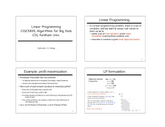
Linear Programming • In linear programming, the goal is to optimize (i.e., maximize or minimize) a linear objective function subject to a set of linear constraints • Many practical optimization problems can be posed within this framework • Efficient algorithms are known for solving linear programs – Linear programming solving packages routinely solve LP instances with thousands of variables and constraints Theory in Programming Practice, Plaxton, Spring 2004

Linear Functions • A linear function of variables x 1 , . . . x n is any function of the form c 0 + � 1 ≤ j ≤ n c j x j where – The c j ’s denote given real numbers – The x j ’s denote real variables • Example: 3 x 1 − 2 x 2 + 10 Theory in Programming Practice, Plaxton, Spring 2004

Linear Objective Function • The objective function is the function that we are striving to maximize or minimize • Suppose our goal is to maximize the linear function 3 x 1 − 2 x 2 + 10 (subject to certain constraints that remain to be specified) • We will get the same result if we drop the constant term and instead simply maximize 3 x 1 − 2 x 2 • Also, note that maximizing 3 x 1 − 2 x 2 is the same as minimizing − 3 x 1 + 2 x 2 • Such a linear objective function is often written in the more compact vector form c T x , where c and x are viewed as n × 1 column vectors, the superscript T denotes transpose, and multiplication corresponds to inner product Theory in Programming Practice, Plaxton, Spring 2004

Linear Constraints • A linear constraint requires that a given linear function be at most, at least, or equal to, a specified real constant – Examples: 3 x 1 − 2 x 2 ≤ 10 ; 3 x 1 − 2 x 2 ≥ 10 ; 3 x 1 − 2 x 2 = 10 • Note that any such linear constraint can be expressed in terms of upper bound (“at most”) constraints – The lower bound constraint 3 x 1 − 2 x 2 ≥ 10 is equivalent to the upper bound constraint − 3 x 1 + 2 x 2 ≤ − 10 – The equality constraint 3 x 1 − 2 x 2 = 10 is equivalent to the upper bound constraints 3 x 1 − 2 x 2 ≤ 10 and − 3 x 1 + 2 x 2 ≤ − 10 Theory in Programming Practice, Plaxton, Spring 2004

Sets of Linear Constraints: Matrix Notation • Suppose we are given a set of m upper bound constraints involving the n variables x 1 , . . . , x n • The constraints can be written in the form Ax ≤ b where A denotes an m × n real matrix, x denotes a column vector of length n (i.e., an n × 1 matrix), and b denotes a column vector of length m – The i th inequality, 1 ≤ i ≤ m , is � 1 ≤ j ≤ n a ij x j ≤ b i • Similarly, a set of lower bounds constraints may be written as Ax ≥ b and a set of equality constraints may be written as Ax = b Theory in Programming Practice, Plaxton, Spring 2004

Nonnegativity Constraints • The special case of a linear constraint that requires a particular variable, say x j , to be nonnegative (i.e., x j ≥ 0 ) is sometimes referred to as a nonnegativity constraint • We will see that such constraints may be handled in a special way within the simplex algorithm, which accounts for their special status – Basically, such constraints are handled implicitly rather than explicitly Theory in Programming Practice, Plaxton, Spring 2004

Standard Form • A linear programming instance is said to be in standard form if it is of the form: Maximize c T x subject to Ax ≤ b and x ≥ 0 • It is relatively straightforward to transform any given LP instance into this form – As noted earlier, a minimization problem can be converted to a maximization problem by negating the objective function – We have already seen how to represent lower bound constraints and equality constraints using upper bound constraints – If a nonnegativity constraint is missing for some variable x j (i.e., x j is “unrestricted”), we can represent x j by x ′ j − x ′′ j where the variables x ′ j and x ′′ j are required to be nonnegative Theory in Programming Practice, Plaxton, Spring 2004

Geometric Interpretation • Suppose we wish to maximize 3 x 1 + 2 x 2 subject to the constraints (1) x 1 + x 2 ≤ 10 (2) x 1 ≤ 8 (3) x 2 ≤ 5 (4) x 1 and x 2 nonnegative • Let’s draw out the feasible region in the plane • Now use a geometric approach to find an optimal solution Theory in Programming Practice, Plaxton, Spring 2004

Simplex Algorithm • In general, the feasible region defined by constraints of the form Ax ≤ b and x ≥ 0 forms a simplex • An optimal solution is guaranteed to occur at some “corner” of the simplex • These “corners” correspond to basic feasible solutions, a notion to be defined a bit later • The simplex algorithm maintains a bfs, and repeatedly moves to an “adjacent” bfs with a higher value for the objective function • The simplex algorithm terminates when it reaches a local optimum – Fortunately, for the linear programming problem, any such local optimum can be proven to also be a global optimum Theory in Programming Practice, Plaxton, Spring 2004

Simplex Algorithm: Performance • In the worst case, the simplex algorithm can take a long time (exponential number of iterations) to converge – Fortunately, only pathological inputs lead to such bad behavior; in practice, the running time of the simplex algorithm is quite good • More sophisticated algorithms (e.g., the ellipsoid algorithm) are known for linear programming that are guaranteed to run in polynomial time Theory in Programming Practice, Plaxton, Spring 2004

Running Example • Maximize 4 x 1 + 5 x 2 + 9 x 3 + 11 x 4 ( c T x ) subject to x 1 + x 2 + x 3 + x 4 ≤ 15 7 x 1 + 5 x 2 + 3 x 3 + 2 x 4 ≤ 120 3 x 1 + 5 x 2 + 10 x 3 + 15 x 4 ≤ 100 ( Ax ≤ b ) and x j ≥ 0 , 1 ≤ j ≤ 4 • An application: – Variable x j denotes the amount of product j to produce – Value c j denotes the profit per unit of product j – Value a ij denotes the amount of raw material i used to produce each unit of product j – Value b i denotes the available amount of raw material i – The objective is to maximize profit Theory in Programming Practice, Plaxton, Spring 2004

Simplex Example • Let x 0 denote the value of the objective function and introduce n = 3 slack variable x 5 , x 6 , x 7 to obtain the following equivalent system • Maximize x 0 subject to the constraints x 0 − 4 x 1 − 5 x 2 − 9 x 3 − 11 x 4 = 0 x 1 + x 2 + x 3 + x 4 + x 5 = 15 7 x 1 + 5 x 2 + 3 x 3 + 2 x 4 + x 6 = 120 3 x 1 + 5 x 2 + 10 x 3 + 15 x 4 + x 7 = 100 • It is easy to see that the above constraints are satisfied by setting x 0 to 0 , setting each slack variable to the corresponding RHS (i.e., x 5 to 15, x 6 to 120, and x 7 to 100), and setting the remaining variables to 0 – Simplex uses this method to obtain an initial feasible solution Theory in Programming Practice, Plaxton, Spring 2004

Basic Feasible Solution • There are four constraints in the system given on the preceding slide • Simplex will consider only solutions with at most four nonzero variables • Such a solution is called a basic feasible solution or bfs • The four variables that are allowed to be nonzero are called the basic variables; the remaining variables are called nonbasic • We view the initial feasible solution mentioned on the previous slide as a bfs with basic variables x 0 = 0 , x 5 = 15 , x 6 = 120 , and x 7 = 100 Theory in Programming Practice, Plaxton, Spring 2004

The High-Level Strategy of the Simplex Algorithm • The algorithm proceeds iteratively; at each iteration, we have a bfs • We also have a system of equations, one for each basic variable, such that the associated basic variable has coefficient 1 and the remaining basic variables have coefficient 0 – In our example, we chose x 0 , x 5 , x 6 , and x 7 as our initial basic variables – Note that our initial system of four equations satisfies the aforementioned conditions • The value of the objective function (i.e., of the variable x 0 ) increases strictly at each iteration • When the algorithm terminates, the current bfs is optimal, i.e., x 0 is maximized Theory in Programming Practice, Plaxton, Spring 2004

A Simplex Iteration • Check a termination condition to see whether the current bfs is optimal; if so, terminate • Apply a particular rule to choose an entering variable , i.e., a nonbasic variable that will become a basic variable after this iteration • Apply a second rule to choose a departing variable , i.e., a basic variable that will become a nonbasic variable after this iteration • Perform a pivot operation to determine a new bfs, and to update the associated system of equations appropriately Theory in Programming Practice, Plaxton, Spring 2004