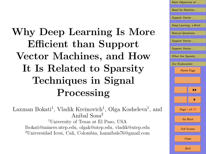
Why Deep Learning Is More Natural Questions Efficient than Support - PowerPoint PPT Presentation

Main Objectives of . . . Need for Machine . . . Support Vector . . . Deep Learning: a Brief . . . Why Deep Learning Is More Natural Questions Efficient than Support Support Vector . . . Support Vector . . . Vector Machines, and How What Are Sparsity . . . Our Explanation It Is Related to Sparsity Home Page Techniques in Signal Title Page Processing ◭◭ ◮◮ ◭ ◮ Laxman Bokati 1 , Vladik Kreinovich 1 , Olga Kosheleva 1 , and Page 1 of 33 Anibal Sosa 2 Go Back 1 University of Texas at El Paso, USA lbokati@miners.utep.edu, olgak@utep.edu, vladik@utep.edu Full Screen 2 Universidad Icesi, Cali, Colombia, hannibals76@gmail.com Close Quit

Main Objectives of . . . Need for Machine . . . 1. Main Objectives of Science and Engineering Support Vector . . . • We want to make our lives better, we want to select Deep Learning: a Brief . . . actions and designs that will make us happier. Natural Questions Support Vector . . . • We want to improve the world so as to increase our Support Vector . . . happiness level. What Are Sparsity . . . • To do that, we need to know: Our Explanation Home Page – what is the current state of the world, and – what changes will occur if we perform different ac- Title Page tions. ◭◭ ◮◮ • Crudely speaking: ◭ ◮ – learning the state of the world and learning what Page 2 of 33 changes will happen is science, while Go Back – using this knowledge to come up with the best ac- Full Screen tions and best designs is engineering. Close Quit

Main Objectives of . . . Need for Machine . . . 2. Need for Machine Learning Support Vector . . . • In some cases, we already know how the world oper- Deep Learning: a Brief . . . ates. Natural Questions Support Vector . . . • E.g., we know that the movement of the celestial bodies Support Vector . . . is well described by Newton’s equations. What Are Sparsity . . . • It is described so well that we can predict, e.g., Solar Our Explanation eclipses centuries ahead. Home Page • In many other cases, however, we do not have such a Title Page good knowledge. ◭◭ ◮◮ • We need to extract the corresponding laws of nature ◭ ◮ from the observations. Page 3 of 33 Go Back Full Screen Close Quit

Main Objectives of . . . Need for Machine . . . 3. Need for Machine Learning (cont-d) Support Vector . . . • In general, prediction means that: Deep Learning: a Brief . . . Natural Questions – we can predict the future value y of the physical Support Vector . . . quantity of interest Support Vector . . . – based on the current and past values x 1 , . . . , x n of What Are Sparsity . . . related quantities. Our Explanation • To be able to do that, we need to have an algorithm Home Page that: Title Page – given the values x 1 , . . . , x n , ◭◭ ◮◮ – computes a reasonable estimate for the desired fu- ◭ ◮ ture value y . Page 4 of 33 Go Back Full Screen Close Quit

Main Objectives of . . . Need for Machine . . . 4. Need for Machine Learning (cont-d) Support Vector . . . • In the past, designing such algorithms was done by Deep Learning: a Brief . . . geniuses: Natural Questions Support Vector . . . – Newton described how to predict the motion of ce- Support Vector . . . lestial bodies, What Are Sparsity . . . – Einstein provided more accurate algorithms, Our Explanation – Schroedinger, in effect, described how to predict Home Page probabilities of different quantum states, etc. Title Page • This still largely remains the domain of geniuses, Nobel ◭◭ ◮◮ prizes are awarded every year for these discoveries. ◭ ◮ • However, now that the computers has become very ef- Page 5 of 33 ficient, they are often used to help. Go Back Full Screen Close Quit

Main Objectives of . . . Need for Machine . . . 5. Need for Machine Learning (cont-d) Support Vector . . . • This use of computers is known as machine learning : Deep Learning: a Brief . . . Natural Questions – we know, in several cases c = 1 , . . . , C , which values y ( c ) corresponded to appropriate values x ( c ) Support Vector . . . 1 , . . . , x ( c ) n ; Support Vector . . . – we want to find an algorithm f ( x 1 , . . . , x n ) for which, What Are Sparsity . . . for all these cases c , we have y ( c ) ≈ f ( x ( c ) 1 , . . . , x ( c ) n ). Our Explanation • The value y may be tomorrow’s temperature in a given Home Page area. Title Page • It may be a binary (0-1) variable deciding, e.g., whether ◭◭ ◮◮ a given email is legitimate or a spam. ◭ ◮ Page 6 of 33 Go Back Full Screen Close Quit

Main Objectives of . . . Need for Machine . . . 6. Machine Learning: a Brief History Support Vector . . . • One of the first successful general machine learning Deep Learning: a Brief . . . techniques was the technique of neural networks . Natural Questions Support Vector . . . • In this technique, we look for algorithms of the type Support Vector . . . � n K � What Are Sparsity . . . � � f ( x 1 , . . . , x n ) = W k · s w ki · x i − w k 0 − W 0 . Our Explanation i =1 k =1 Home Page • Here, a non-linear function s ( z ) is called an activation Title Page function , and values w ki and W k knows as weights . ◭◭ ◮◮ • As the function s ( z ), researchers usually selected the ◭ ◮ so-called sigmoid function Page 7 of 33 1 s ( z ) = 1 + exp( − z ) . Go Back Full Screen • This algorithm emulates a 3-layer network of biological neurons – the main brain cells doing data processing. Close Quit

Main Objectives of . . . Need for Machine . . . 7. Machine Learning: a Brief History (cont-d) Support Vector . . . • In the first layer, we have input neurons that read the Deep Learning: a Brief . . . inputs x 1 , . . . , x n . Natural Questions Support Vector . . . • In the second layer – called a hidden layer – we have Support Vector . . . K neurons each of which: What Are Sparsity . . . – first generates a linear combination of the input Our Explanation n signals: z k = � w ki · x i − w k 0 Home Page i =1 – and then applies an appropriate nonlinear function Title Page s ( z ) to z k , resulting in a signal y k = s ( z k ). ◭◭ ◮◮ • The processing by biological neurons is well described ◭ ◮ by the sigmoid activation function. Page 8 of 33 • This is the reason why this function was selected for Go Back artificial neural networks in the first place. Full Screen • After that, in the final output layer, the signals y k from the neurons in the hidden layer are combined. Close Quit

Main Objectives of . . . Need for Machine . . . 8. Machine Learning: a Brief History (cont-d) Support Vector . . . K Deep Learning: a Brief . . . • The linear combination � W k · y k − W 0 is returned as Natural Questions k =1 the output. Support Vector . . . Support Vector . . . • A special efficient algorithm – backpropagation – was developed to train the corresponding neural network. What Are Sparsity . . . Our Explanation • This algorithm finds the values of the weights that pro- Home Page vide the best fit for the observation results x ( c ) 1 , . . . , x ( c ) n , y ( c ) . Title Page ◭◭ ◮◮ ◭ ◮ Page 9 of 33 Go Back Full Screen Close Quit

Main Objectives of . . . Need for Machine . . . 9. Support Vector Machines (SVM): in Brief Support Vector . . . • Later, in many practical problem, a different technique Deep Learning: a Brief . . . became more efficient: the SVM technique. Natural Questions Support Vector . . . • Let us explain this technique on the example of a binary Support Vector . . . classification problem, i.e., a problem in which: What Are Sparsity . . . – we need to classify all objects (or events) into one Our Explanation of two classes, Home Page – based on the values x 1 , . . . , x n of the corresponding Title Page parameters ◭◭ ◮◮ • In such problems, the desired output y has only two ◭ ◮ possible values; this means that: Page 10 of 33 – the set of all possible values of the tuple x = ( x 1 , . . . , x n ) Go Back – is divided into two non-intersecting sets S 1 and S 2 corresponding to each of the two classes. Full Screen Close Quit

Main Objectives of . . . Need for Machine . . . 10. Support Vector Machines (cont-d) Support Vector . . . • We can thus come up with a continuous f-n f ( x 1 , . . . , x n ) Deep Learning: a Brief . . . such that f ( x ) ≥ 0 for x ∈ S 1 and f ( x ) ≤ 0 for x ∈ S 2 . Natural Questions Support Vector . . . • As an example of such a function, we can take f ( x ) = Support Vector . . . def d ( x, S 2 ) − d ( x, S 1 ), where d ( x, S ) = inf s ∈ S d ( x, s ). What Are Sparsity . . . • If x ∈ S , then d ( x, s ) = 0 for s = x thus d ( x, S ) = 0. Our Explanation Home Page • For points x ∈ S 1 , we have d ( x, S 1 ) = 0 but usually d ( x, S 2 ) > 0, thus f ( x ) = d ( x, S 2 ) − d ( x, S 1 ) > 0. Title Page ◭◭ ◮◮ • For points x ∈ S 2 , we have d ( x, S 2 ) = 0 while, in gen- eral, d ( x, S 1 ) > 0, thus f ( x ) = d ( x, S 2 ) − d ( x, S 1 ) < 0 . ◭ ◮ • In some cases, there exists a linear function that sepa- Page 11 of 33 n rates the classes: f ( x 1 , . . . , x n ) = a 0 + � a i · x i . Go Back i =1 Full Screen • In this case, there exist efficient algorithms for finding the corresponding coefficients a i . Close Quit