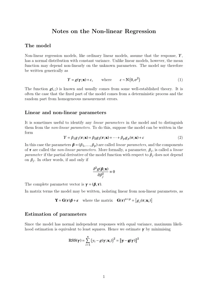
Notes on the Non-linear Regression The model Non-linear regression - PDF document
Notes on the Non-linear Regression The model Non-linear regression models, like ordinary linear models, assume that the response, Y , has a normal distribution with constant variance. Unlike linear models, however, the mean function may depend
Notes on the Non-linear Regression The model Non-linear regression models, like ordinary linear models, assume that the response, Y , has a normal distribution with constant variance. Unlike linear models, however, the mean function may depend non-linearly on the unknown parameters. The model my therefore be written generically as 0 , σ 2 � � where (1) Y = g ( γ ; x ) + ε , ε ∼ N The function g ( , ;) is known and usually comes from some well-established theory. It is often the case that the fixed part of the model comes from a deterministic process and the random part from homogeneous measurement errors. Linear and non-linear parameters It is sometimes useful to identify any linear parameters in the model and to distinguish them from the non-linear parameters . To do this, suppose the model can be written in the form (2) Y = β 1 g 1 ( τ ; x ) + β 2 g 2 ( τ ; x ) +···+ β p g p ( τ ; x ) + ε In this case the parameters β = ( β 1 ,..., β p ) are called linear parameters , and the components of τ are called the non-linear parameters . More formally, a parameter, β j , is called a linear parameter if the partial derivative of the model function with respect to β j does not depend on β j . In other words, if and only if ∂ 2 g ( β ; x ) ≡ 0 ∂β 2 j The complete parameter vector is γ = ( β , τ ) . In matrix terms the model may be written, isolating linear from non-linear parameters, as G ( τ ) n × p = � � where the matrix Y = G ( τ ) β + ε g j ( τ ; x i ) Estimation of parameters Since the model has normal independent responses with equal variance, maximum likeli- hood estimation is equivalent to least squares. Hence we estimate γ by minimising n � 2 = � 2 � � � � RSS( γ ) = y i − g ( γ ; x i ) � y − g ( γ ) i = 1 1
Solution locus and tangent space It is useful to have a geometric understanding of this problem. Let Γ be the set of all possible values of the unknown parameter vector, γ p × 1 . The p − dimensional surface S in n − dimensional sample space defined by ⊂ R n � � S = g ( γ ) | γ ∈ Γ is sometimes called the “solution locus”. It is the known set in which the true mean vector lies. The points within S are uniquely indexed by the parameter vector γ , which therefore defines a coordinate system within S . The response vector, y n × 1 , is also in R n , and the estimation problem amounts to finding the vector in S closest to the observation vector, y in the sense of Euclidean distance. The vector itself is the estimated mean and the coordinates of the vector are the least squares estimates of the parameters. Let γ (0) be an initial approximate to the least squares estimate vector, ˆ γ , and expand the model function in a first order Taylor series about γ (0) : � � g ( γ ; x i ) = g ( γ (0) ; x i ) + ∂ g 1 ) +···+ ∂ g � γ = γ (0) ( γ 1 − γ (0) ( γ p − γ (0) � � p ) + “smaller order terms” � � ∂γ 1 ∂γ p � γ = γ (0) The vectors 1 = ∂ g � p = ∂ g � g (0) � γ = γ (0) ,..., g (0) � � � � ∂γ 1 ∂γ p � γ = γ (0) define the tangent space to the solution locus, S , at the point defined by γ (0) . Iterative approximation An iterative method for finding the least squares estimates, equivalent to the usual Newton- Raphson scheme, is as follows: 1. Begin with an initial approximation, γ (0) , obtained by any convenient method. 2. Calculate the tangent vectors to S at the point defined by γ (0) , that is, g (0) 1 ,..., g (0) p . � � g (0) 1 ,..., g (0) 3. Regress y − g ( γ (0) ) on G = using ordinary least squares, and call the p coefficient vector δ (0) . γ is then γ (1) = γ (0) + δ (0) . 4. The new approximation to ˆ 5. Iterate the process until, (hopefully), convergence to the MLE, γ ( i ) → ˆ γ . 6. The usual estimate of σ 2 is then � 2 � � � y − g ( ˆ γ ) = RSS( ˆ γ ) s 2 = n − p n − p by analogy with the linear regression case, (though it is neither the maximum likeli- hood estimate, nor a REML estimate). 2
A geometrical interpretation of the algorithm is as follows: ❼ Start at a point on the solution locus defined by the initial approximation. ❼ Calculate a basis for the tangent space at the initial approximation. The tangent space is a linear space which shares the same coordinate system as the solution locus itself. ❼ Project the response vector orthogonally onto the tangent space. ❼ The coordinates of the projection in the tangent space define a new approximation. ❼ Go to the point on the solution locus corresponding to the coordinates of the point on the tangent space, and repeat the process. ❼ If the process converges, the projection onto the tangent space should be at the same point as where he tangent space itself touches the solution locus, which implies that the point on the solution locus closest to the response vector, in the sense of Euclidean distance, has been obtained. Inference and diagnostic checks Most of the inferential procedures with non-linear regression are based on the assumption that the approximating tangential regression at the MLE is adequate, and linear regression theory is used. Thus nested models are tested using F − tests, as if they were linear regres- sions. So called “profiling” of the likelihood (or least squares) surface can offer some check on these assumptions, by giving some insight into deviation from the expected quadratic behaviour. The usual summary output from a non-linear least squares fit shows much the same infor- mation as for a linear regression. The same diagnostic checks apply for non-linear regression as apply for linear. Plots of residuals against fitted values, and normal scores plots are just as important in non-linear regression as in linear. Other measures, such as Cook’s distances and leverage, however, can only really be applied to the approximating tangential linear regression, and there are few ready-made tools for doing this. It would be easily possible, however, and this is a gap in the suite of R facilities that could usefully be plugged. Notes on the software Non-linear regression is a very general suite of models and, unlike generalized linear models, there are no reasonable automatic methods for generating good starting values for the iterative process. The fitting algorithms generally need a lot of input from the user to ensure the processes work. The R fitting function, nls , provides facilities to assist the user in this. In particular 1. the deriv function allows the user to create a function to specify the form of the non-linear regression, and the partial derivatives of the model function with respect 3
to the parameters as well. Providing the partial derivatives allows the algorithm to find the tangent space directly. If these are not supplied, the algorithm has to find the tangent space by numerical differences, which can be a less stable process; 2. the selfStart function allows the user to include an automatic starting procedure in the model specification function as well as first derivatives. This not only makes the process simpler to use, but if the starting value procedure is good enough, it can make the iterative process safer and quicker. Several self-starting model functions have already been written for particular classes of non-linear regression models commonly in use. These are located in the stats package, along with nls itself. > require(stats) [1] TRUE > objects("package:stats", patt = "^SS.*") [1] "SSasymp" "SSasympOff" "SSasympOrig" "SSbiexp" "SSD" [6] "SSfol" "SSfpl" "SSgompertz" "SSlogis" "SSmicmen" [11] "SSweibull" 3. Linear parameters have the property that, if the non-linear parameters are known (or fixed), they may then be estimated by linear least squares. If there are many linear parameters, it can be very important to take advantage of this simplification. The plinear algorithm in nls allows this. Using this algorithm the model funcion is supplied as a matrix, the columns of which the linear parameters multiply. That is, as the matrix G ( τ ) defined here in an earlier section. 4
Recommend
More recommend
Explore More Topics
Stay informed with curated content and fresh updates.
