EKF, UKF Pieter Abbeel UC Berkeley EECS Many slides adapted from - PowerPoint PPT Presentation

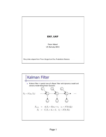
EKF, UKF Pieter Abbeel UC Berkeley EECS Many slides adapted from Thrun, Burgard and Fox, Probabilistic Robotics

Kalman Filter Kalman Filter = special case of a Bayes’ filter with dynamics model and n sensory model being linear Gaussian: 2 -1

Kalman Filtering Algorithm n At time 0: n For t = 1, 2, … n Dynamics update: n Measurement update:

Nonlinear Dynamical Systems n Most realistic robotic problems involve nonlinear functions: n Versus linear setting: 4

Linearity Assumption Revisited y y p(y) x p(x) x 5

Linearity Assumption Revisited y y p(y) x p(x) x 6

Non-linear Function y y p(y) x p(x) “Gaussian of p(y)” has mean and variance of y under p(y) x 7

EKF Linearization (1) 8

EKF Linearization (2) p(x) has high variance relative to region in which linearization is accurate. 9

EKF Linearization (3) p(x) has small variance relative to region in which linearization is accurate. 10

EKF Linearization: First Order Taylor Series Expansion n Dynamics model: for x t “close to” µ t we have: n Measurement model: for x t “close to” µ t we have: 11

EKF Linearization: Numerical n Numerically compute F t column by column: n Here e i is the basis vector with all entries equal to zero, except for the i’t entry, which equals 1. n If wanting to approximate F t as closely as possible then ² is chosen to be a small number, but not too small to avoid numerical issues

Ordinary Least Squares n Given: samples {(x (1) , y (1) ), (x (2) , y (2) ), …, (x (m) , y (m) )} n Problem: find function of the form f(x) = a 0 + a 1 x that fits the samples as well as possible in the following sense:

Ordinary Least Squares n Recall our objective: n Let’s write this in vector notation: n , giving: n Set gradient equal to zero to find extremum: (See the Matrix Cookbook for matrix identities, including derivatives.)

Ordinary Least Squares n For our example problem we obtain a = [4.75; 2.00] a 0 + a 1 x

Ordinary Least Squares 26 24 22 20 30 20 0 10 20 30 40 10 n More generally: 0 n In vector notation: n , gives: n Set gradient equal to zero to find extremum (exact same derivation as two slides back):

Vector Valued Ordinary Least Squares Problems n So far have considered approximating a scalar valued function from samples {(x (1) , y (1) ), (x (2) , y (2) ), …, (x (m) , y (m) )} with n A vector valued function is just many scalar valued functions and we can approximate it the same way by solving an OLS problem multiple times. Concretely, let then we have: n In our vector notation: n This can be solved by solving a separate ordinary least squares problem to find each row of

Vector Valued Ordinary Least Squares Problems n Solving the OLS problem for each row gives us: n Each OLS problem has the same structure. We have

Vector Valued Ordinary Least Squares and EKF Linearization n Approximate x t+1 = f t ( x t , u t ) with affine function a 0 + F t x t by running least squares on samples from the function: {( x t(1) , y (1) = f t ( x t(1) , u t ), ( x t(2) , y (2) = f t ( x t(2) , u t ), …, ( x t(m) , y (m) = f t ( x t(m) , u t )} n Similarly for z t+1 = h t ( x t )

OLS and EKF Linearization: Sample Point Selection n OLS vs. traditional (tangent) linearization: OLS traditional (tangent)

OLS Linearization: choosing samples points n Perhaps most natural choice: n n reasonable way of trying to cover the region with reasonably high probability mass

Analytical vs. Numerical Linearization n Numerical (based on least squares or finite differences) could give a more accurate “regional” approximation. Size of region determined by evaluation points. n Computational efficiency: n Analytical derivatives can be cheaper or more expensive than function evaluations n Development hint: n Numerical derivatives tend to be easier to implement n If deciding to use analytical derivatives, implementing finite difference derivative and comparing with analytical results can help debugging the analytical derivatives

EKF Algorithm n At time 0: n For t = 1, 2, … n Dynamics update: n Measurement update:

EKF Summary n Highly efficient: Polynomial in measurement dimensionality k and state dimensionality n : O(k 2.376 + n 2 ) n Not optimal! n Can diverge if nonlinearities are large! n Works surprisingly well even when all assumptions are violated! 35

Linearization via Unscented Transform EKF UKF 36

UKF Sigma-Point Estimate (2) EKF UKF 37

UKF Sigma-Point Estimate (3) EKF UKF 38

UKF Sigma-Point Estimate (4)

[Julier and Uhlmann, 1997] UKF intuition why it can perform better Assume we know the distribution over X and it has a mean \bar{x} n Y = f(X) n EKF approximates f by first order and ignores higher-order terms n UKF uses f exactly, but approximates p(x). n

Original unscented transform Picks a minimal set of sample points that match 1 st , 2 nd and 3 rd moments n of a Gaussian: \bar{x} = mean, P xx = covariance, i à i’th column, x 2 < n n · : extra degree of freedom to fine-tune the higher order moments of n the approximation; when x is Gaussian, n+ · = 3 is a suggested heuristic L = \sqrt{P_{xx}} can be chosen to be any matrix satisfying: n n L L T = P xx [Julier and Uhlmann, 1997]

Beyond scope of course, just A crude preliminary investigation of whether we can get EKF to match including for completeness. UKF by particular choice of points used in the least squares fitting

Self-quiz n When would the UKF significantly outperform the EKF? y x n Analytical derivatives, finite-difference derivatives, and least squares will all end up with a horizontal linearization à they’d predict zero variance in Y = f(X)

Unscented Kalman filter n Dynamics update: n Can simply use unscented transform and estimate the mean and variance at the next time from the sample points n Observation update: n Use sigma-points from unscented transform to compute the covariance matrix between x t and z t . Then can do the standard update.

[Table 3.4 in Probabilistic Robotics]

UKF Summary n Highly efficient: Same complexity as EKF, with a constant factor slower in typical practical applications n Better linearization than EKF: Accurate in first two terms of Taylor expansion (EKF only first term) + capturing more aspects of the higher order terms n Derivative-free: No Jacobians needed n Still not optimal!