Non-Stationary Time Series, Cointegration and Spurious Regression - PDF document

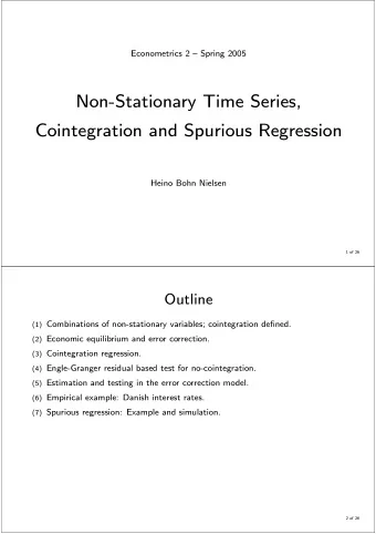
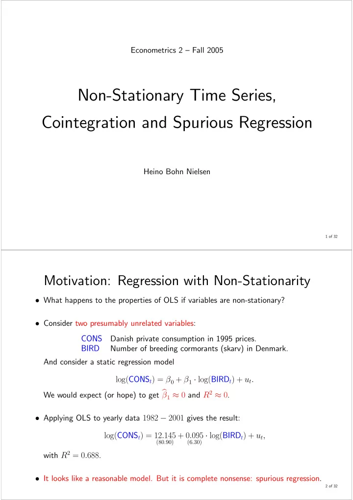
Econometrics 2 — Fall 2005 Non-Stationary Time Series, Cointegration and Spurious Regression Heino Bohn Nielsen 1 of 32 Motivation: Regression with Non-Stationarity • What happens to the properties of OLS if variables are non-stationary? • Consider two presumably unrelated variables: CONS Danish private consumption in 1995 prices. BIRD Number of breeding cormorants (skarv) in Denmark. And consider a static regression model log( CONS t ) = β 0 + β 1 · log( BIRD t ) + u t . We would expect (or hope) to get b β 1 ≈ 0 and R 2 ≈ 0 . • Applying OLS to yearly data 1982 − 2001 gives the result: log( CONS t ) = 12 . 145 (80 . 90) + 0 . 095 (6 . 30) · log( BIRD t ) + u t , with R 2 = 0 . 688 . • It looks like a reasonable model. But it is complete nonsense: spurious regression. 2 of 32

• The variables are non-stationary. The residual, u t , is non-stationary and standard results for OLS do not hold. • In general, regression models for non-stationary variables give spurious results. Only exception is if the model eliminates the stochastic trends to produce stationary residuals: Cointegration. • For non-stationary variables we should always think in terms of cointegration. Only look at regression output if the variables cointegrate. Consumption and breeding birds, logs Regression residuals (cons on birds) Consumption 13.2 Number of breeding birds 1 13.1 0 13.0 -1 12.9 1985 1990 1995 2000 1985 1990 1995 2000 3 of 32 Outline De fi nitions and concepts: (1) Combinations of non-stationary variables; Cointegration de fi ned. (2) Economic equilibrium and error correction. Engle-Granger two-step cointegration analysis: (3) Static regression for cointegrated time series. (4) Residual based test for no-cointegration. (5) Models for the dynamic adjustment. Cointegration analysis based on dynamic models: (6) Estimation in the unrestricted ADL or ECM model. (7) PcGive test for no-cointegration. What if variables do not cointegrate? (8) Spurious regression revisited. 4 of 32

Cointegration De fi ned • Let X t = ( X 1 t X 2 t ) 0 be two I(1) variables, i.e. they contain stochastic trends: X t X 1 t = i =1 � 1 i + initial value + stationary process X t X 2 t = i =1 � 2 i + initial value + stationary process. • In general, a linear combination of X 1 t and X 2 t will also have a random walk. De fi ne β = ( 1 − β 2 ) 0 and consider the linear combination: ¢ µ ¶ ¡ 1 − β 2 X 1 t Z t = β 0 X t = = X 1 t − β 2 X 2 t X 2 t X t X t = i =1 � 1 i − β 2 i =1 � 2 i + initial value + stationary process. • Important exception: There exist a β , so that Z t is stationary: We say that X 1 t and X 2 t co-integrate with cointegration vector β . 5 of 32 Remarks: (1) Cointegration occurs if the stochastic trends in X 1 t and X 2 t are the same so they cancel, P t i =1 � 1 i = β 1 · P t i =1 � 2 i . This is called a common trend. (2) You can think of an equation eliminating the random walks in X 1 t and X 2 t : X 1 t = µ + β 2 X 2 t + u t . ( † ) If u t is I(0) (mean zero) then β = ( 1 − β 2 ) 0 is a cointegrating vector. (3) The cointegrating vector is only unique up to a constant factor. 0 X t = bβ 0 X t for b 6 = 0 . We can choose a normalization If β 0 X t ∼ I(0). Then so is e β µ ¶ µ ¶ − e 1 β 1 e β = β = . or − β 2 1 This corresponds to di ff erent variables on the left hand side of ( † ) (4) Cointegration is easily extended to more variables. ¡ X 1 t X 2 t · · · ¢ 0 cointegrate if The variables in X t = X pt Z t = β 0 X t = X 1 t − β 2 · X 2 t − ... − β p · X pt ∼ I(0). 6 of 32

Cointegration and Economic Equilibrium • Consider a regression model for two I(1) variables, X 1 t and X 2 t , given by X 1 t = µ + β 2 X 2 t + u t . ( ∗ ) The term, u t , is interpretable as the deviation from the relation in ( ∗ ). • If X 1 t and X 2 t cointegrate, then the deviation u t = X 1 t − µ − β 2 X 2 t is a stationary process with mean zero. Shocks to X 1 t and X 2 t have permanent e ff ects. X 1 t and X 2 t co-vary and u t ∼ I(0). We can think of ( ∗ ) as de fi ning an equilibrium between X 1 t and X 2 t . • If X 1 t and X 2 t do not cointegrate, then the deviation u t is I(1). There is no natural interpretation of ( ∗ ) as an equilibrium relation. 7 of 32 Empirical Example: Consumption and Income • Time series for log consumption, C t , and log income, Y t , are likely to be I(1). De fi ne a vector X t = ( C t Y t ) 0 . • Consumption and income are cointegrated with cointegration vector β = ( 1 − 1 ) 0 if the (log-) consumption-income ratio, µ ¶ C t Z t = β 0 X t = ( 1 − 1 ) = C t − Y t , Y t is a stationary process. The consumption-income ratio is an equilibrium relation. Income ratio, log ( C t ) − log ( Y t ) Consumption and income, logs 0.00 Income Consumption 6.25 -0.05 -0.10 6.00 -0.15 1970 1980 1990 2000 1970 1980 1990 2000 8 of 32

How is the Equilibrium Sustained? • There must be forces pulling X 1 t or X 2 t towards the equilibrium. • Famous representation theorem: X 1 t and X 2 t cointegrate if and only if there exist an error correction model for either X 1 t , X 2 t or both. • As an example, let Z t = X 1 t − β 2 X 2 t be a stationary relation between I(1) variables. Then there exists a stationary ARMA model for Z t . Assume for simplicity an AR(2): Z t = θ 1 Z t − 1 + θ 2 Z t − 2 + � t , θ (1) = 1 − θ 1 − θ 2 > 0 . This is equivalent to ( X 1 t − β 2 X 2 t ) = θ 1 ( X 1 t − 1 − β 2 X 2 t − 1 ) + θ 2 ( X 1 t − 2 − β 2 X 2 t − 2 ) + � t X 1 t = β 2 X 2 t + θ 1 X 1 t − 1 − θ 1 β 2 X 2 t − 1 + θ 2 X 1 t − 2 − θ 2 β 2 X 2 t − 2 + � t , or ∆ X 1 t = β 2 ∆ X 2 t + θ 2 β 2 ∆ X 2 t − 1 − θ 2 ∆ X 1 t − 1 − (1 − θ 1 − θ 2 ) { X 1 t − 1 − β 2 X 2 t − 1 } + � t . In this case we have a common-factor restriction. That is not necessarily true. 9 of 32 More on Error-Correction • Cointegration is a system property. Both variables could error correct, e.g.: ∆ X 1 t = δ 1 + Γ 11 ∆ X 1 t − 1 + Γ 12 ∆ X 2 t − 1 + α 1 ( X 1 t − 1 − β 2 X 2 t − 1 ) + � 1 t ∆ X 2 t = δ 2 + Γ 21 ∆ X 1 t − 1 + Γ 22 ∆ X 2 t − 1 + α 2 ( X 1 t − 1 − β 2 X 2 t − 1 ) + � 2 t , • We may write the model as the so-called vector error correction model, µ ¶ µ ¶ µ ¶ µ ¶ µ ¶ µ ¶ ∆ X 1 t δ 1 Γ 11 Γ 12 ∆ X 1 t − 1 α 1 � 1 t = + + ( X 1 t − 1 − β 2 X 2 t − 1 )+ , ∆ X 2 t δ 2 Γ 21 Γ 22 ∆ X 2 t − 1 α 2 � 2 t or simply ∆ X t = δ + Γ∆ X t − 1 + αβ 0 X t − 1 + � t . • Note that β 0 X t − 1 = X 1 t − 1 − β 2 X 2 t − 1 appears in both equations. • For X 1 t to error correct we need α 1 < 0 . For X 2 t to error correct we need α 2 > 0 . 10 of 32

Consider a simple model for two cointegrated variables: µ ¶ µ ¶ µ ¶ ∆ X 1 t − 0 . 2 � 1 t = ( X 1 t − 1 − X 2 t − 1 ) + . ∆ X 2 t 0 . 1 � 2 t β ' X t = X 1 t − X 2 t (A) Two cointegrated variables (B) Deviation from equilibrium, X 1 t 0 X 2 t 2.5 -5 0.0 -10 -2.5 0 20 40 60 80 100 0 20 40 60 80 100 β ' X t (C) Speed of adjustment of (D) Cross-plot 12.5 X 1 t × X 2 t 0 10.0 7.5 -5 5.0 2.5 -10 0.0 X 100 -2.5 11 of 32 0 20 40 60 80 100 -12.5 -10.0 -7.5 -5.0 -2.5 0.0 OLS Regression with Cointegrated Series • In the cointegration case there exists a β 2 so that the error term, u t , in X 1 t = µ + β 2 X 2 t + u t . ( ∗∗ ) is stationary. • OLS applied to ( ∗∗ ) gives consistent results, so that b β 2 → β 2 for T → ∞ . • Note that consistency is obtained even if potential dynamic terms are neglected. This is because the stochastic trends in X 1 t and X 2 t dominate. We can even get consistent estimates in the reverse regression X 2 t = δ + γ 1 X 1 t + v t . • Unfortunately, it turns out that b β 2 is not asymptotically normal in general. The normal inferential procedures do not apply to b β 2 ! We can use ( ∗∗ ) for estimation—not for testing. 12 of 32

Super-Consistency • For stationary series, the variance of b β 1 declines at a rate of T − 1 . • For cointegrated I(1) series, the variance of b β 1 declines at a faster rate of T − 2 . • Intuition: If b β 1 = β 1 then u t is stationary. If b β 1 6 = β 1 then the error is I(1) and will have a large variance. The ’information’ on the parameter grows very fast. Stationary, T=50 Stationary, T=100 Stationary, T=500 30 30 30 20 20 20 10 10 10 0 0 0 0.5 1.0 1.5 0.5 1.0 1.5 0.5 1.0 1.5 Non-Stationary, T=50 Non-Stationary, T=500 Non-Stationary, T=100 30 30 30 20 20 20 10 10 10 0 0 0 0.5 1.0 1.5 0.5 1.0 1.5 0.5 1.0 1.5 13 of 32 Test for No-Cointegration, Known β 1 • Suppose that X 1 t and X 2 t are I(1). Also assume that β = ( 1 − β 2 ) 0 is known. • The series cointegrate if Z t = X 1 t − β 2 X 2 t is stationary. • This can be tested using an ADF unit root test, e.g. the test for H 0 : π = 0 in X k ∆ Z t = δ + ∆ Z t − i + πZ t − 1 + η t . i =1 The usual DF critical values apply to t π =0 . • Note, that the null, H 0 : π = 0 , is a unit root, i.e. no cointegration. 14 of 32