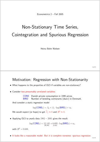
Non-Stationary Time Series, Cointegration and Spurious Regression - PDF document

Econometrics 2 — Spring 2005 Non-Stationary Time Series, Cointegration and Spurious Regression Heino Bohn Nielsen 1 of 26 Outline (1) Combinations of non-stationary variables; cointegration de fi ned. (2) Economic equilibrium and error correction. (3) Cointegration regression. (4) Engle-Granger residual based test for no-cointegration. (5) Estimation and testing in the error correction model. (6) Empirical example: Danish interest rates. (7) Spurious regression: Example and simulation. 2 of 26

Combinations of Non-Stationary Variables • Let W t = ( Y t X t ) 0 be two I(1) variables, i.e. they contain stochastic trends: X t Y t = Y 0 + i =1 � i + stationary process X t X t = X 0 + i =1 η i + stationary process. In general, a linear combination will also have a random walk component: ¢ µ ¶ ¡ 1 − β 1 Y t Z t = β 0 W t = = Y t − β 1 · X t X t X t X t = Y 0 − β 1 · X 0 + i =1 � i − β 1 · i =1 η i + stationary process. • Important exception: There exist a β = ( 1 − β 1 ) 0 , so that Z t is stationary. In this case we say that Y t and X t co-integrate with cointegration vector β . • Cointegration occurs if the stochastic trends in Y t and X t are the same: X t X t i =1 � i = β 1 · i =1 η i . 3 of 26 Cointegration and Economic Equilibrium • Consider a regression model for two I(1) variables, Y t and X t , given by Y t = β 0 + β 1 X t + � t . ( ∗ ) The term, � t , is interpretable as the deviation from the relation in ( ∗ ). • If Y t and X t cointegrate, then the deviation � t = Y t − β 0 − β 1 X t is a stationary process with attractor zero. Shocks to Y t and X t have permanent e ff ects; but Y t and X t co-vary so that � t returns to zero. We think of ( ∗ ) as de fi ning an equilibrium between Y t and X t . • If Y t and X t do not cointegrate, then the deviation � t is I(1). There is no natural interpretation of ( ∗ ) as an equilibrium relation. 4 of 26

Empirical Example: Consumption and Income • Time series for log consumption, C t , and log income, Y t , are likely to be I(1). De fi ne a vector W t = ( C t Y t ) 0 . • Consumption and income are cointegrated with cointegration vector β = ( 1 − 1 ) 0 if the (log-) consumption-income ratio, µ ¶ C t Z t = β 0 W t = ( 1 − 1 ) = C t − Y t , Y t is a stationary process. The consumption-income ratio is an equilibrium relation. Income ratio, log ( C t ) − log ( Y t ) Consumption and income, logs 0.00 Income Consumption 6.25 -0.05 -0.10 6.00 -0.15 1970 1980 1990 2000 1970 1980 1990 2000 5 of 26 How is the Equilibrium Sustained? • There must be forces pulling Y t or X t towards the attractor. • Famous representation theorem: Y t and X t cointegrate if and only if there exist an error correction model for either Y t , X t or both. • As an example, let Z t = Y t − β 1 X t be a stationary relation between I(1) variables. Then there exists a stationary AR model for Z t . Assume for simplicity an AR(2): Z t = θ 1 Z t − 1 + θ 2 Z t − 2 + v t , θ (1) = 1 − θ 1 − θ 2 > 0 . This is equivalent to ( Y t − β 1 X t ) = θ 1 ( Y t − 1 − β 1 X t − 1 ) + θ 2 ( Y t − 2 − β 1 X t − 2 ) + v t Y t = β 1 X t + θ 1 Y t − 1 − θ 1 β 1 X t − 1 + θ 2 Y t − 2 − θ 2 β 1 X t − 2 + v t , or ∆ Y t = β 1 ∆ X t + θ 2 β 1 ∆ X t − 1 − θ 2 ∆ Y t − 1 − (1 − θ 1 − θ 2 ) { Y t − 1 − β 1 X t − 1 } + v t . In this case we have a common-factor restriction. That is not necessarily true. 6 of 26

OLS Regression with Cointegrated Series • In the cointegration case there exists a β 1 so that the error term, � t , in Y t = α + β 1 X t + � t . ( ∗∗ ) is stationary. • OLS applied to ( ∗∗ ) gives consistent results, so that b β 1 → β 1 for T → ∞ . • Note that consistency is obtained even if potential dynamic terms are neglected. This is because the stochastic trends in Y t and X t dominate. We can even get consistent estimates in the reverse regression X t = δ + γ 1 Y t + η t . • Unfortunately, it turns out that b β 1 is not asymptotically normal in general. The normal inferential procedures do not apply to b β 1 ! We can use ( ∗∗ ) for estimation—not for testing. 7 of 26 Super-Consistency • For stationary series, the variance of b β 1 declines at a rate of T − 1 . • For cointegrated I(1) series, the variance of b β 1 declines at a faster rate of T − 2 . • Intuition: If b β 1 = β 1 then � t is stationary. If b β 1 6 = β 1 then the error is I(1) and will have a large variance. The ’information’ on the parameter grows very fast. Stationary, T=50 Stationary, T=100 Stationary, T=500 30 30 30 20 20 20 10 10 10 0 0 0 0.5 1.0 1.5 0.5 1.0 1.5 0.5 1.0 1.5 Non-Stationary, T=50 Non-Stationary, T=500 Non-Stationary, T=100 30 30 30 20 20 20 10 10 10 0 0 0 0.5 1.0 1.5 0.5 1.0 1.5 0.5 1.0 1.5 8 of 26

Test for No-Cointegration, Known β 1 • Suppose that we know that Y t and X t are I(1). Assume that β 1 is known. • The series cointegrate, with cointegration vector β = ( 1 − β 1 ) , if Z t = Y t − β 1 X t is stationary. • This can be tested using an ADF unit root test, e.g. the test for H 0 : π = 0 in p − 1 X ∆ Z t = δ + ∆ Z t − i + πZ t − 1 + η t . i =1 The usual DF critical values apply to t π =0 . • Note, that the null, H 0 : π = 0 , is a unit root, i.e. no cointegration. 9 of 26 Test for No-Cointegration, Estimated β 1 • Engle-Granger (1987) two-step procedure. • If β 1 is unknown, it can be (super-consistently) estimated in Y t = β 0 + β 1 X t + � t . ( ∗ ∗ ∗ ) b β = ( 1 − b β 1 ) is a cointegration vector if b � t is a stationary process. • This can be tested using a DF unit root test, e.g. the test for H 0 : π = 0 in p − 1 X ∆ b ∆ b � t − i + π b � t = � t − 1 + η t . i =1 The critical value for t π =0 depends on the deterministic regressors in ( ∗ ∗ ∗ ). • The fact that b β 1 is estimated also change the critical values. OLS in ( ∗ ∗ ∗ ) minimizes the variance of b � t . Look ’as stationary as possible’. Critical value depends on the number of regressors. 10 of 26

0.6 Estimated parameters in cointegrating regression (with constant in the regression (***)) 7 6 5 4 3 2 1 0.5 DF(constant) 0.4 N(0,1) 0.3 0.2 0.1 -8 -7 -6 -5 -4 -3 -2 -1 0 1 2 3 4 5 11 of 26 • Critical values for the Dickey-Fuller test for no-cointegration are given by: Case 1: A constant term in ( ∗ ∗ ∗ ). Number of variables Signi fi cance level incl. Y t 1% 5% 10% 2 − 3 . 90 − 3 . 34 − 3 . 04 3 − 4 . 29 − 3 . 74 − 3 . 45 4 − 4 . 64 − 4 . 10 − 3 . 81 5 − 4 . 96 − 4 . 42 − 4 . 13 Case 2: A constant and a trend in ( ∗ ∗ ∗ ). Number of variables Signi fi cance level incl. Y t 1% 5% 10% 2 − 4 . 32 − 3 . 78 − 3 . 50 3 − 4 . 66 − 4 . 12 − 3 . 84 4 − 4 . 97 − 4 . 43 − 4 . 15 5 − 5 . 25 − 4 . 72 − 4 . 43 12 of 26

Dynamic Modelling • Given the estimated cointegrating vector we can de fi ne the error correction term � t = Y t − b β 0 − b ecm t = b β 1 X t , which is, per de fi nition, a stationary stochastic variable. • Since b β 1 converges to β 1 very fast we can treat it as a fi xed number and formulate an error correction model conditional on ecm t , i.e. ∆ Y t = δ + φ 0 ∆ X t + φ 1 ∆ X t − 1 + θ ∆ Y t − 1 − γ · ecm t − 1 + v t . • Given cointegration, all terms are stationary, and normal inference applies to δ , φ 0 , φ 1 , θ , and γ . 13 of 26 Estimation of β In the ECM • The estimator of β 1 from a static regression is super-consistent, but often biased due to ignored dynamics. • An alternative estimator is based on an unrestricted error correction model, e.g. ∆ Y t = δ + θ ∆ Y t − 1 + φ 0 ∆ X t + φ 1 ∆ X t − 1 + γ 1 Y t − 1 + γ 2 X t − 1 + v t , ( # ) which is equivalent to the unrestricted ADL regression Y t = δ + α 1 Y t − 1 + α 2 Y t − 2 + κ 1 X t + κ 2 X t − 1 + κ 3 X t − 2 + v t . An estimate of β 1 can be found as the parameter in the long-run solutions: β 1 = − b γ 2 b = ( b κ 1 + b κ 2 + b κ 3 ) / (1 − b α 1 − b α 2 ) . b γ 1 • The main advantage is that the analysis is undertaken in a well-speci fi ed model. The approach is optimal if only Y t error corrects. 14 of 26

Testing for No-Cointegration in the ECM • Due to representation theorem, the null hypothesis of no-cointegration corre- sponds to the null of no-error-correction. • Several tests have been designed in this spirit. • The most convenient is the so-called PcGive test for no-cointegration. It is based on the unrestricted ECM: ∆ Y t = δ + θ ∆ Y t − 1 + φ 0 ∆ X t + φ 1 ∆ X t − 1 + γ 1 Y t − 1 + γ 2 X t − 1 + � t , ( # ) and tests the hypothesis H 0 : γ 1 = 0 against the cointegration alternative, γ 1 < 0 . • The distribution of the t − ratio, b γ 1 t γ 1 =0 = γ 1 ) , SE ( b depends on the deterministic terms and the number of regressors in ( # ). 15 of 26 • Critical values for the PcGive test for no-cointegration are given by: Case 1: A constant term in ( # ). Number of variables Signi fi cance level incl. Y t 1% 5% 10% 2 − 3 . 79 − 3 . 21 − 2 . 91 3 − 4 . 09 − 3 . 51 − 3 . 19 4 − 4 . 36 − 3 . 76 − 3 . 44 5 − 4 . 59 − 3 . 99 − 3 . 66 Case 2: A constant and a trend in ( # ). Number of variables Signi fi cance level incl. Y t 1% 5% 10% 2 − 4 . 25 − 3 . 69 − 3 . 39 3 − 4 . 50 − 3 . 93 − 3 . 62 4 − 4 . 72 − 4 . 14 − 3 . 83 5 − 4 . 93 − 4 . 34 − 4 . 03 16 of 26