Binary Logistic Regression In ordinary linear regression with - PowerPoint PPT Presentation

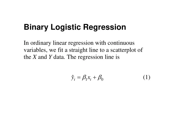
Binary Logistic Regression In ordinary linear regression with continuous variables, we fit a straight line to a scatterplot of the X and Y data. The regression line is = β + β (1) ˆ i y x 1 0 i

It is important to remember that, when fitting the scatterplot, we estimate an equation for (a) predicting a Y score from the X score, but also for μ (b) estimating the conditional mean = for a | y x a given value a . In Psychology 310, you may recall that we exploited this fact to perform hypothetical distribution calculations for weight given height.

0 β + x β 1 = y x | μ x y x | μ

Binary Data as “Censored” Information Suppose that the X-Y data are bivariate normal, but that the scores on Y are censored in the following way. There is a threshold or critical value y , and C if an underlying y value exceeds the threshold, the y = , otherwise y = . observed score is 1 0 How will this censoring affect the conditional mean?

The Mean of a Binary Censored Normal Variable Recall that, with a binary variable, the mean is y = . So the equal to the probability that 1 conditional mean is simply the probability that > | . y y x C

In this plot, we have reversed the usual positions of x and y. Notice that, as x increases, the predicted values of y increase in a straight line, and so does the conditional mean of y for that value of x. The conditional normal distributions are represented. The area above y is shaded in. This area is not C only the probability that the binary “censored” version of y will be equal to 1, it is also the conditional mean of the censored (binary) version of y . If you examine the size of the shaded areas, you see the key fact. The relationship between the conditional mean of the censored y and x is not linear!

We can easily plot the relationship, as in the following example. Suppose the original data are in standard score form, and the population correlation is 0.60. Then the regression line is = μ = .6 (2) ˆ y x | y x The formula for the conditional mean of the censored version of y ( y* ) is

− .6 y x > = π = − Φ C Pr( | ) ( ) 1 ( ) y y x x c − 2 1 .6 − .6 y x = − Φ C 1 ( ) (3) .8 − .6 x y = Φ C ( ) .8 Note that if the cutoff point is at 0, the equation becomes ( ) > = μ = Φ Pr( | ) .75 (4) y y x x *| c y x

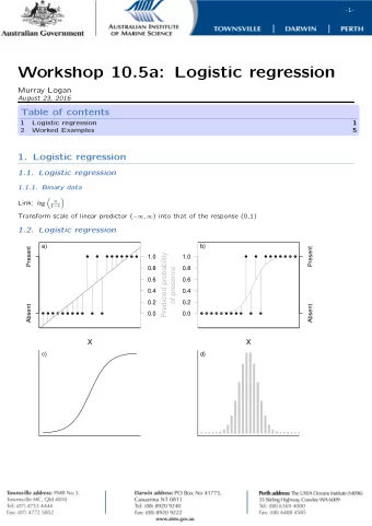
So the plot of the conditional mean of y* versus x will have the same shape as the cumulative distribution function of the normal curve. 1 0.8 0.6 0.4 0.2 -3 -2 -1 1 2 3

So there are several reasons why we would not want to use simple linear regression to predict the π conditional mean ( ) , say as x π = β + β ( ) (5) x x 1 0 First, we realize that the relationship is almost certainly not going to be linear over the whole range of x , although it may well be quite linear over a significant middle portion of the graph. Second, Equation (5) can generate improper values, i.e., values greater than 1 or less than 0.

Third, the standard assumption of equality of variance of conditional distributions is clearly not true, since, as you recall from our study of the binomial, [ ] = π − π Var( *| ) ( ) 1 ( ) (6) y x x x which varies as a function of x. π So rather than fitting a linear function to ( ) , we x should fit a nonlinear function. Examining Equation (3) again, we see that it can be written in the form

( ) π = Φ α + β ( ) (7) x x Since Φ is invertible, we can write [ ] − Φ π = α + β 1 ( ) (8) x x This is known as a probit model. It is a special case of a Generalized Linear Model (GLM), which, broadly speaking, is a linear model for a transformed mean of a variable that has a distribution in the natural exponential family .

Binomial Logit Models Suppose we simply assume that the response variable has a binary distribution, with probabilities π and 1 π − for 1 and 0, respectively. Then the probability density can be written − π = π − π 1 y y ( ; ) (1 ) f y ) [ ] ( = − π π − π y 1 /(1 ) (9) π ⎛ ⎞ ( ) = − π ⎜ ⎟ 1 exp log1 y − π ⎝ ⎠

y = given x are a Now, suppose the log-odds of 1 linear function of x , i.e., π ( ) x [ ] π = = α + β logit ( ) log1 (10) x x − π ( ) x The logit function is invertible, and so ( ) α + β exp x π = + ( ) (11) x ( ) α + β 1 exp x

Interpreting Logistic Parameters In the above simple case, if we fit this model to data, how would we interpret the estimates of the model parameters? Exponentiating both sides of Equation (10) shows that the odds are an exponential function of x . The odds increase multiplicatively by e β for every unit increase in x . β = So, for example, if .5 , the odds are multiplied by 1.64 for every unit increase in x.

π Also, if we take the derivative of ( ) with respect x [ ] βπ − π to x , we find that it is equal to ( ) 1 ( ) . So x x locally, the probability of x is increasing by [ ] βπ − π ( ) 1 ( ) for each unit increase in x . x x This in turn implies that the steepest slope is at π = = − α β ( ) 1/2 , at which / . In toxicology, x x this is called LD , because it is the dose at which 50 the probability of death is 1/2. The intercept parameter is of less interest.

Example. Agresti (2002, Chapter 5) presents a simple example, predicting whether a female crab has a “satellite,” i.e., a male living within a defined short distance, on the basis of biological characteristics of the female.

1. Load data into SPSS, create new variables “has_sat” by computing sat>0. 2. Analyze � Regression � Binary Logistic. Results. Variables in the Equation B S.E. Wald df Sig. Exp(B) Step W .497 .102 23.887 1 .000 1.644 a 1 Constant -12.351 2.629 22.075 1 .000 .000 a. Variable(s) entered on step 1: W.

π H x L 1 0.8 0.6 0.4 0.2 Width H x L 22 24 26 28 30 32 34

Variables in the Equation 95.0% C.I.for EXP(B) B S.E. Wald df Sig. Exp(B) Lower Upper a Step 1 RACE .055 .289 .037 1 .848 1.057 .600 1.861 AZT -.719 .279 6.651 1 .010 .487 .282 .841 Constant -1.074 .263 16.670 1 .000 .342 a. Variable(s) entered on step 1: RACE, AZT.

Casewise List Observed Temporary Variable Selected Predicted Status a Case SYMPTOMS Predicted Group Resid ZResid 1 S 1** .150 0 .850 2.384 2 S 0 .150 0 -.150 -.419 3 S 1** .265 0 .735 1.664 4 S 0 .265 0 -.265 -.601 5 S 1** .143 0 .857 2.451 6 S 0 .143 0 -.143 -.408 7 S 1** .255 0 .745 1.711 8 S 0 .255 0 -.255 -.585 a. S = Selected, U = Unselected cases, and ** = Misclassified cases.