Multiple Regression Review Instructor: G. William Schwert 275-2470 - PDF document

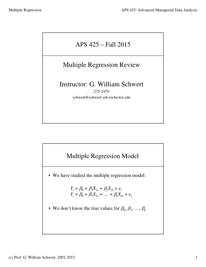
Multiple Regression APS 425- Advanced Managerial Data Analysis APS 425 – Fall 2015 Multiple Regression Review Instructor: G. William Schwert 275-2470 schwert@schwert.ssb.rochester.edu Multiple Regression Model • We have studied the multiple regression model: Y i =  0 +  1 X 1 i +  2 X 2 i + e i Y i =  0 +  1 X 1 i + … +  n X ni + e i • We don’t know the true values for  0 ,  1 , …,  n (c) Prof. G. William Schwert, 2001-2015 1

Multiple Regression APS 425- Advanced Managerial Data Analysis Multiple Regression Model • Given a sample, we find, as before, estimators b 0 , b 1 , …, b n , by minimizing the sum of squared prediction errors: ^  e i 2 =  ( Y i – Y i ) 2 , where Y i = b 0 + b 1 X 1 i + … + b n X ni ^ ^ • The estimators b 0 , b 1 , …, b n are unbiased, consistent, and efficient estimators of the population parameters  0 ,  1 , …,  n if the following six assumptions are satisfied Multiple Regression Model • Six Assumptions: – E( e i ) = 0 – the model is correctly specified, i.e., Y i =  0 +  1 X 1 i + … +  n X ni + e i – Corr( X ki , e i ) = 0 for all i , k – e i has a normal distribution – Var( e i ) =  = a constant – Corr( e i , e j ) = 0 for all i , j • Hence, if these assumptions are satisfied, the estimators b 0 , b 1 , …, b n provide accurate information about the values of the population parameters  0 ,  1 , …,  n (c) Prof. G. William Schwert, 2001-2015 2

Multiple Regression APS 425- Advanced Managerial Data Analysis Example: Wine Prices & Weather • The Excel spreadsheet A425_WINE.XLSX contains market prices for a collection of 13 high quality Bordeaux wines (not including Château Petrus or Château Mouton Rothschild, both of which have prices that are often out of line with their “quality”) from different vintages (years). All prices (PRICE) are expressed relative to the prices of the 1961 vintage, which is renowned for being the best during this period. So, for example, the portfolio of 13 1989 vintage Bordeaux wines costs 23% as much as the same wines from the 1961 vintage. Example: Wine Prices & Weather • The data were provided by Professor Orley Ashenfelter of Princeton University, publisher of Liquid Assets , a wine newsletter that provides current auction prices for wines and forecasts quality of new wine vintages [http://www.liquidasset.com]. • There are no prices for wines after 1989 because these wines were not mature at the time these data were prepared. One of the goals of this exercise is to construct a method of forecasting the prices (or values) of these wines. (c) Prof. G. William Schwert, 2001-2015 3

Multiple Regression APS 425- Advanced Managerial Data Analysis Example: Wine Prices & Weather • The weather variables for the Bordeaux region of France are some of the main determinants of the quality of wine. Harvest rainfall (HARVRAIN, the sum of rainfall from September and October, in mm) is important because if it rains too much during the harvest season then the wines will be too watery or too diluted. The better vintages have dry harvest periods and are said to be more concentrated. Summer temperature (SUMTEMP, the average temperature from April through August, in degrees centigrade) is also important because the hotter weather is necessary for the grapes to fully ripen. Riper, sweeter fruit produces a better quality wine. Example: Wine Prices & Weather • Riper, sweeter fruit produces a better quality wine. Winter rainfall (WINTRAIN, the sum of rainfall from November through June, in mm) is important because wetter weather is good for the grape vines early in the growing season. The average temperature during the harvest season (SEPTEMP) is also included because some people suspect that wines that are “soft and easy drinking” are made when it was hot during the September when the grapes were being picked. (c) Prof. G. William Schwert, 2001-2015 4

Multiple Regression APS 425- Advanced Managerial Data Analysis Example: Wine Prices & Weather • Age is also an important determinant of the price of wine. The reason for this is largely because the quality of wines improves with age. A typical wine might take 10 years to mature and continues to improve in quality beyond that point. Of course, it is also true that the price must be increasing with age, otherwise consumers would not buy wines when they were young (they could put their money in the bank instead and buy the wines when they were older). • A quick glance at the data reveals that 1961, 1953, and 1959 are among the hottest and driest years for Bordeaux wines, and also have the highest relative prices. Of course, these are also some of the older wines in our data. Wine Prices & Weather: Questions • Are the theoretical predictions about the effect of weather on wine quality supported by these data? • If you think about wine as an investment, is there any evidence that it pays to buy wine when it is young and store it, or should you spend your money on wine after it has matured? • Prof. Ashenfelter originally analyzed these data using the 1952-80 sample period and become so famous in wine circles that the New York Times wrote an extensive story about his equation in their weekend edition (see abstract below). Is there any evidence that the model for wine prices changes when you include the additional data from 1981-89? (c) Prof. G. William Schwert, 2001-2015 5

Multiple Regression APS 425- Advanced Managerial Data Analysis Wine Prices & Weather: Questions • Often wine connoisseurs do tastings of Bordeaux wines when they are still developing in large oak barrels and try to forecast what the wine will be like when it is drinkable. For example, Robert Parker has become famous because people have come to trust his skill at evaluating wines in this way. I have included Parker’s ratings of the major Bordeaux regions for each year from 1970-2009 from his web page [http://www.erobertparker.com/info/VintageChart.pdf] and then averaged them to create a vintage quality measure called “PARKER” in the spreadsheet. Do Parker’s quality rankings help explain prices? • How would you create an index of quality for different vintages using only weather information? How does it compare with Parker’s ratings? • How would you forecast prices from 1990-2010? Initial Regression • Start with simple regression that tries to explain price as a function of rain during the harvest (HARVRAIN) and during the prior winter (WINTRAIN), and temperature during the growing season (SUMTEMP) and during the harvest season (SEPTEMP) (c) Prof. G. William Schwert, 2001-2015 6

Multiple Regression APS 425- Advanced Managerial Data Analysis Initial Regression • Start with simple regression that tries to explain price as a function of rain during the harvest (HARVRAIN) and during the prior winter (WINTRAIN), and temperature during the growing season (SUMTEMP) and during the harvest season (SEPTEMP) Results, 1952-89 • Note that one of these coefficient estimates has a t-statistic larger than 2 in absolute value • What does this mean? • Is the overall regression significant? • How would you test this? (c) Prof. G. William Schwert, 2001-2015 7

Multiple Regression APS 425- Advanced Managerial Data Analysis Results, 1952-89 • It looks like the residuals (blue line on the bottom) have higher mean and variance in the early years • They seem to be trending down and their amplitude is larger in the early data => Try adding the time variable to reflect that fact that older wines cost more (otherwise, why would anyone store them for drinking later?) Results, 1952-89 • It looks like adding TIME to reflect to different age of the vintages was important (t-stat of –5.39) • Adjusted R 2 increases from 23.3% to 53.5% • The weather variables seem to make sense: higher temperatures are associated with better (higher priced) wine; rain before the growing season is good, but during harvest is bad (c) Prof. G. William Schwert, 2001-2015 8

Multiple Regression APS 425- Advanced Managerial Data Analysis Results, 1952-89 • We have fixed the trend, but it still looks like the residuals (blue line on the bottom) have higher variance in the early years => Try log transformation for price Scatter plots of Price or Log(price) vs. Time • The log(price) plot looks like it will have less heteroskedasticity (c) Prof. G. William Schwert, 2001-2015 9

Multiple Regression APS 425- Advanced Managerial Data Analysis Log(Price) Results, 1952-89 Adjusted R 2 in the log • model is a little higher than in the “raw” model (61.1% vs. 53.5%) • Coefficients change because of the change in functional form, but the qualitative conclusions are the same Log(Price) Results, 1952-89 • These plots look much better: amplitude of the residuals is similar throughout 1952-89 • This is because using log(price) is essentially like looking at percentage changes, rather than absolute changes, in wine prices • % changes are more likely to have the same distribution across long time periods (c) Prof. G. William Schwert, 2001-2015 10