Announcements Grades for the first midterm are posted, solutions to - PowerPoint PPT Presentation

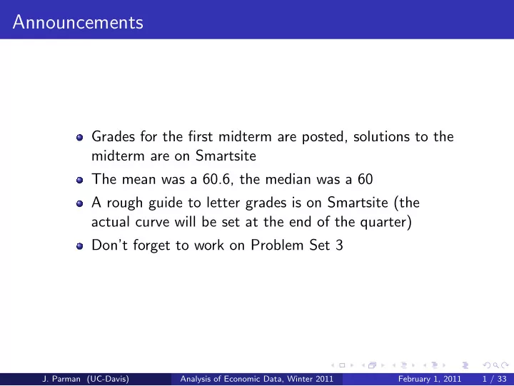
Announcements Grades for the first midterm are posted, solutions to the midterm are on Smartsite The mean was a 60.6, the median was a 60 A rough guide to letter grades is on Smartsite (the actual curve will be set at the end of the quarter) Don’t forget to work on Problem Set 3 J. Parman (UC-Davis) Analysis of Economic Data, Winter 2011 February 1, 2011 1 / 33

Midterm 1 Grade Distribution 35 30 25 Frequency 20 15 10 10 5 0 0 5 10 15 20 25 30 35 40 45 50 55 60 65 70 75 80 85 90 95 100 Midterm 1 score J. Parman (UC-Davis) Analysis of Economic Data, Winter 2011 February 1, 2011 2 / 33

Reviewing the Regression Line y i = b 1 + b 2 x i ˆ ˆ y i : predicted value for Y for individual i x i : observed value of X for individual i b 1 : intercept (predicted value of Y when X equals 0) b 2 : slope (predicted ∆ Y for a one unit increase in X ) J. Parman (UC-Davis) Analysis of Economic Data, Winter 2011 February 1, 2011 3 / 33

Reviewing the Regression Line Recall that the residual is: ε i = y i − ˆ y i We wanted to choose b 1 and b 2 to minimize the average of the squared residuals: � y i ) 2 min ( y i − ˆ b 1 , b 2 Replacing ˆ y with the equation for the regression line makes this: � ( y i − b 1 − b 2 x i ) 2 min b 1 , b 2 J. Parman (UC-Davis) Analysis of Economic Data, Winter 2011 February 1, 2011 4 / 33

Reviewing the Regression Line If you work through the math, you come up with the following two equations giving b 1 and b 2 : � n i =1 ( x i − ¯ x )( y i − ¯ y ) b 2 = � n x ) 2 i =1 ( x i − ¯ b 1 = ¯ y − b 2 ¯ x Notice that the first equation looks very similar to our variance and covariance formulas, we can rewrite b 2 as: � s yy b 2 = s xy = r xy s xx s xx J. Parman (UC-Davis) Analysis of Economic Data, Winter 2011 February 1, 2011 5 / 33

Calculating the Regression Line To calculate b 2 and b 1 yourself: Calculate the covariance of X and Y using the 1 covariance function in Excel Calculate the variance of X using the variance function 2 in Excel Calculate b 2 by dividing the covariance of X and Y by 3 the variance of X Calculate b 1 by subtracting ¯ x times the b 2 you just 4 found from ¯ y (¯ x and ¯ y can be calculated with the average function in Excel) To have Excel calculate b 2 and b 1 , use ’Regression’ from the ’Data Analysis’ choices J. Parman (UC-Davis) Analysis of Economic Data, Winter 2011 February 1, 2011 6 / 33

Assessing How Good the Fit Is We found the best fit for the regression line (according to our definition) This doesn’t mean that we have a perfect fit; many data points will not be on the line We would like to know just how good the fit is, how well does the line fit the data? To answer this, we can use either the standard error of the regression or the R-squared J. Parman (UC-Davis) Analysis of Economic Data, Winter 2011 February 1, 2011 7 / 33

The Standard Error of the Regression Think back to the residuals: y i − ˆ y i One way to check how good the fit is is to see how big the residuals are on average This is what the standard error of the regression does: n 1 s 2 � y i ) 2 e = ( y i − ˆ n − 2 i =1 The smaller the standard error of the regression is, the closer the fitted values are to the actual data for y J. Parman (UC-Davis) Analysis of Economic Data, Winter 2011 February 1, 2011 8 / 33

The R-Squared The standard error of the regression depends on the units that Y is measured in The R 2 provides a standardized measure of how good the fit is The idea behind the R 2 is to determine how much of the observed variation in y can be explained by the regression on x To do this, we need to measure the total variation in y and the amount of the variation that isn’t explained by the regression These two measures are the total sum of squares and the error (or residual) sum of squares , respectively J. Parman (UC-Davis) Analysis of Economic Data, Winter 2011 February 1, 2011 9 / 33

The R-Squared The total sum of squares: n � y ) 2 TSS = ( y i − ¯ i =1 The error sum of squares: n � y i ) 2 ESS = ( y i − ˆ i =1 The R-squared: R 2 = 1 − ESS TSS J. Parman (UC-Davis) Analysis of Economic Data, Winter 2011 February 1, 2011 10 / 33

The R-Squared The R 2 will always be between 0 and 1 An R 2 of 1 means a perfect fit, x perfectly predicts y An R 2 of 0 means no fit, variation in x can’t explain any of the variation in y One interpretation of the R 2 value is that it is the percentage of the variation in y explained by variation in x With a little algebra, you can show that R 2 is the square of r xy The higher the correlation of two variables, the greater the R 2 will be J. Parman (UC-Davis) Analysis of Economic Data, Winter 2011 February 1, 2011 11 / 33

Regressing Weight on Height Regression Statistics SUMMARY OUTPUT: Weight as dependent variable Multiple R 0.532681203 R Square 0.283749264 Adjusted R Square 0.282871505 Standard Error 29.49983204 Observations 818 ANOVA ANOVA df SS MS F Significance F Regression 1 281318.8979 281318.8979 323.2658446 3.84342E-61 Residual 816 710115.9139 870.2400905 Total 817 991434.8117 Coefficients Standard Error t Stat P-value Lower 95% Upper 95% Intercept Intercept -165.605738 18.65570156 165 605738 18 65570156 -8.87695044 8 87695044 4 30095E 18 4.30095E-18 -202.224555 202 224555 -128.986921 128 986921 height 4.968722683 0.276353423 17.97959523 3.84342E-61 4.426275353 5.511170013 J. Parman (UC-Davis) Analysis of Economic Data, Winter 2011 February 1, 2011 12 / 33

Assessing the R-squared In general, we’d like R 2 to be large but a low R 2 doesn’t necessarily mean we have nothing of interest R 2 will tend to be high when: Looking at certain time series data in economics Looking at data from controlled experiments (especially in the physical sciences) When the outcome is only dependent on a handful of observable variables R 2 will tend to be low when: Looking at certain cross-sectional data in economics (especially wages, employment outcomes, productivity, etc.) Looking at data where there are important but unobservable variables Looking at poorly measured data J. Parman (UC-Davis) Analysis of Economic Data, Winter 2011 February 1, 2011 13 / 33

An Example of a Low R-Squared Regression Statistics Summary Output: Lost works days in past year Multiple R 0.402129 R Square 0.161708 Adjusted R Square 0.128176 Standard Error 85.63869 Observations 27 ANOVA ANOVA df SS MS F ignificance F Regression 1 35368.39 35368.39 4.822534 0.037585 Residual 25 183349.6 7333.985 Total 26 218718 Coefficientsandard Erro t Stat P-value Lower 95%Upper 95% Lower 95.0% Upper 95.0% Intercept Intercept 44 92542 44.92542 34 04049 34.04049 1.319764 1 319764 0 198872 0.198872 -25.18229 25 18229 115 0331 115.0331 -25.18229 25 18229 115 0331 115.0331 Days smoked per month 4.245225 1.933139 2.196027 0.037585 0.263851 8.2266 0.263851 8.2266 J. Parman (UC-Davis) Analysis of Economic Data, Winter 2011 February 1, 2011 14 / 33

An Example of a Low R-Squared 400 400 400 Days of work missed due to illness ssed due to illness Days of work missed due to illness 350 350 350 y = 4.2452x + 44.925 y = 4.2452x + 44.925 y = 4.2452x + 44.925 300 300 300 R² = 0.1617 R² = 0.1617 R² = 0.1617 250 250 250 200 200 200 150 150 100 100 50 50 0 0 0 0 5 5 10 10 15 15 20 20 25 25 30 30 35 35 Days per month that person smoked J. Parman (UC-Davis) Analysis of Economic Data, Winter 2011 February 1, 2011 15 / 33

An Example of a High R-Squared Regression Statistics Summary output: Daily high temperature Multiple R 0.972705 R Square R Square 0.946155 0.946155 Adjusted R 0.946006 Standard E 2.042726 Observatio 363 ANOVA df SS MS F ignificance F Regression 1 26469.32 26469.32 6343.409 4E ‐ 231 Residual 361 1506.355 4.172728 Total 362 27975.67 Coefficients tandard Erro t Stat P ‐ value Lower 95% Upper 95% Lower 95.0% Upper 95.0% Intercept 5.981077 0.129348 46.24032 9.7E ‐ 154 5.726707 6.235446 5.726707 6.235446 Low tempe 1 103883 Low tempe 1.103883 0 01386 0.01386 79 64552 79.64552 4E ‐ 231 4E 231 1 076627 1.076627 1 13114 1.13114 1 076627 1.076627 1 13114 1.13114 J. Parman (UC-Davis) Analysis of Economic Data, Winter 2011 February 1, 2011 16 / 33

An Example of a High R-Squared 35 30 es h temperature (degree 25 20 y = 1.103x + 5.981 celcius) 15 R² = 0.946 10 5 5 Daily high 0 ‐ 15 ‐ 10 ‐ 5 0 5 10 15 20 25 ‐ 5 ‐ 10 Daily low temperature (degrees celcius) J. Parman (UC-Davis) Analysis of Economic Data, Winter 2011 February 1, 2011 17 / 33

Recapping the Regression Line 7 7 7 y = 0.11x + 0.3066 y = 0.11x + 0.3066 y = 0.11x + 0.3066 6 6 6 ns Annual salary, $ millions Annual salary, $ millions R² = 0.4192 R² = 0 4192 R² = 0.4192 5 5 4 4 3 3 2 2 1 0 0 5 10 15 20 25 30 35 Points per game J. Parman (UC-Davis) Analysis of Economic Data, Winter 2011 February 1, 2011 18 / 33

Recapping the Regression Line SUMMARY OUTPUT: ln(salary) regressed on points per game Regression Statistics R Square 0.373151498 Observations 272 ANOVA df SS MS F Regression 1 78.69467035 78.69467 160.72608 Residual 270 132.1973423 0.48962 Total 271 210.8920127 Coefficients Standard Error t Stat P-value Intercept -0.885888855 0.08479455 -10.44747 1.114E-21 points 0.091561535 0.007222206 12.67778 3.268E-29 J. Parman (UC-Davis) Analysis of Economic Data, Winter 2011 February 1, 2011 19 / 33