Assessing Model Fit Our model has assumptions: mean 0 errors, - PowerPoint PPT Presentation

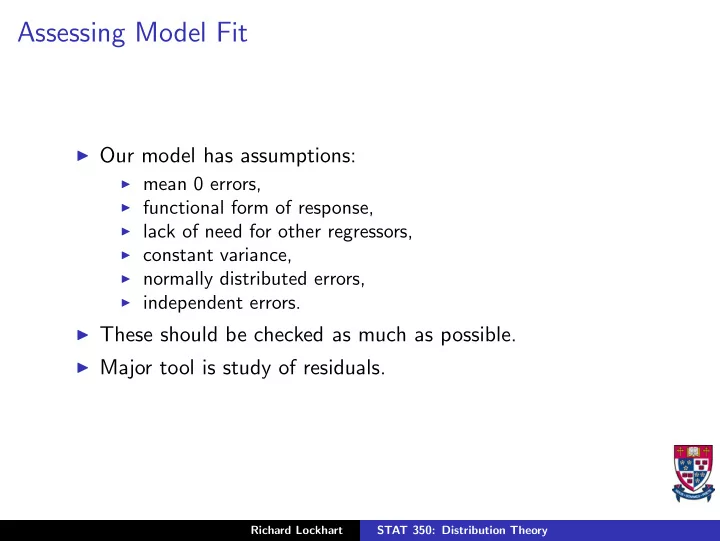
Assessing Model Fit ◮ Our model has assumptions: ◮ mean 0 errors, ◮ functional form of response, ◮ lack of need for other regressors, ◮ constant variance, ◮ normally distributed errors, ◮ independent errors. ◮ These should be checked as much as possible. ◮ Major tool is study of residuals. Richard Lockhart STAT 350: Distribution Theory

Residual Analysis Definition : The residual vector whose entries are called “fitted residuals” or “errors” is ǫ = Y − X ˆ ˆ β. ◮ Examine residual plots to assess quality of model. ◮ Plot residuals ˆ ǫ i against each x i , i.e. against S i and F i . ◮ Plot residuals against other covariates, particularly those deleted from model. ◮ Plot residuals against ˆ µ i = fitted value. ◮ Plot residuals squared against all above. ◮ Make Q-Q plot of residuals. Richard Lockhart STAT 350: Distribution Theory

Look For ◮ Curvature — suggesting need of x 2 or non-linear model. ◮ Heteroscedasticity. ◮ Omitted variables. ◮ Non-normality. Richard Lockhart STAT 350: Distribution Theory

Example Here is a page of plots: Residual vs Sand Residual vs Fibre • • • • 4 4 • • • • 2 • 2 • • • Residual Residual • • 0 • 0 • • • • • • • • • -2 • -2 • • • • • -4 -4 • • 0 5 10 15 20 25 30 0 10 20 30 40 50 Sand Content (%) Fibre Content (%) Residual vs Fitted Q-Q Plot • • • • 4 4 • • • • • 2 • 2 • • • Residual Residual • • 0 • 0 • • • • • • • • • • • • -2 -2 • • • • -4 -4 • • 64 66 68 70 72 74 -2 -1 0 1 2 Fitted Value Quantiles of Standard Normal Richard Lockhart STAT 350: Distribution Theory

Q-Q Plots ◮ Used to check normal assumption for the errors. ◮ Plot order statistics of residuals against quantiles of N (0 , 1): a Q-Q plot : ˆ ǫ (1) < ˆ ǫ (2) < · · · < ˆ ǫ ( n ) are the ˆ ǫ 1 , . . . , ˆ ǫ n arranged in increasing order — called “order statistics”. Also s 1 < · · · < s n are “Normal scores”. They are defined by the equation i P ( N (0 , 1) ≤ s i ) = n + 1 ◮ Plot of s i versus ˆ ǫ i should be near straight line for normal errors. Richard Lockhart STAT 350: Distribution Theory

Conclusions from plots ◮ Q-Q plot is reasonably straight. So normality is OK and t and F tests should work well. ◮ The plot of residual versus fitted values is more or less OK. ◮ Warning : don’t look too hard for patterns; you will find them where they aren’t. ◮ The plot of residual versus Sand is ok. ◮ The plot of residual versus Fibre has mostly positive residuals for the middle values of Fibre suggesting a quadratic pattern. Richard Lockhart STAT 350: Distribution Theory

Consequences ◮ So, we compare Y = β 0 + β 1 S + β 3 F + ǫ and Y = β 0 + β 1 S + β 3 F + β 4 F 2 + ǫ ◮ Use t test on β 4 to test H o : β 4 = 0 in second model. ◮ We find ˆ β 4 = − 0 . 00373 σ ˆ ˆ β 4 = 0 . 001995 t = − 0 . 00373 0 . 001995 = − 1 . 87 based on 14 degrees of freedom. Richard Lockhart STAT 350: Distribution Theory

More discussion ◮ So we get the marginally not significant P value 0.08. ◮ Conclusion: evidence of need for the F 2 term is weak. ◮ We might want more data if the “optimal” Fibre content is needed. ◮ Notice as always: statistics does not eliminate uncertainty but rather quantifies it. Richard Lockhart STAT 350: Distribution Theory

More formal model assessment tools 1. Fit larger model: test for non-zero coefficients. 2. We did this to compare linear to full quadratic model. 3. Look for outlying residuals. 4. Look for influential observations. Richard Lockhart STAT 350: Distribution Theory

Standardized / studentized residuals ◮ Standardized residual is ˆ ǫ i / ˆ σ . ◮ Recall that ǫ ∼ MVN (0 , σ 2 ( I − H )) ˆ ◮ It follows that ǫ i ∼ N (0 , σ 2 (1 − h ii )) ˆ where h ii is the ii th diagonal entry in H . ◮ Jargon : We call h ii the leverage of case i . ◮ We see that ˆ ǫ i σ √ 1 − h ii ∼ N (0 , 1) Richard Lockhart STAT 350: Distribution Theory

Internally Studentized Residuals ◮ Replace σ with the obvious estimate and find that ˆ ǫ i σ √ 1 − h ii ∼ N (0 , 1) ˆ provided that n is large. ◮ Called an internally studentized or standardized residual. ◮ SUGGESTION: look for studentized residuals larger than about 2. ◮ The original standardized residuals are also often used for this. ◮ The h ii add up to the trace of the hat matrix = p . ◮ Average h is p / n which should be small so usually √ 1 − h ii near 1. Richard Lockhart STAT 350: Distribution Theory

Comments ◮ Warning : the N (0 , 1) approximation requires normal errors. ◮ Criticism of internally standardized residuals: if model is bad particularly at point i then including point i pulls the fit towards Y i , inflates ˆ σ and makes the badness hard to see. ◮ Coming soon: eliminate Y i from estimate of σ to compute slightly different residual. Richard Lockhart STAT 350: Distribution Theory

Outlier Plot • • • • • • • • • • • • • • • • • • • • • • • • • • • • • • • • • • • • •• • • • • • • • • • • • • • • •• • • • • • • • • • • • • • • • • • • • • • • • • • • • • • • • • • • • • • • • • • • • • • • • Richard Lockhart STAT 350: Distribution Theory

Deleted Residuals ◮ Suggestion: for each point i delete point i , refit the model, predict Y i . ◮ Call the prediction ˆ Y i ( i ) where the ( i ) in the subscript shows which point was deleted. ◮ Then get case deleted residuals Y i − ˆ Y i ( i ) Richard Lockhart STAT 350: Distribution Theory

Standardized Residuals For insurance data residuals after various model fits: data insure; infile ’insure.dat’ firstobs=2; input year cost; code = year - 1975.5 ; proc glm data=insure; model cost = code ; output out=insfit h=leverage p=fitted r=resid student=isr press=press rstudent=esr; run ; proc print data=insfit ; run; proc glm data=insure; model cost = code code*code code*code*code ; output out=insfit3 h=leverage p=fitted r=resid student=isr press=press rstudent=esr; run ; Richard Lockhart STAT 350: Distribution Theory

proc print data=insfit3 ; run; proc glm data=insure; model cost = code code*code code*code*code code*code*code*code code*code*code*code*code; output out=insfit5 h=leverage p=fitted r=resid student=isr press=press rstudent=esr; run ; proc print data=insfit5 ; run; Richard Lockhart STAT 350: Distribution Theory

Linear Fit Output OBS YEAR COST CODE LEVERAGE FITTED RESID ISR PRESS ESR 1 1971 45.13 -4.5 0.34545 42.5196 2.6104 0.36998 3.9881 0.34909 2 1972 51.71 -3.5 0.24848 48.8713 2.8387 0.37550 3.7773 0.35438 3 1973 60.17 -2.5 0.17576 55.2229 4.9471 0.62485 6.0020 0.59930 4 1974 64.83 -1.5 0.12727 61.5745 3.2555 0.39960 3.7302 0.37758 5 1975 65.24 -0.5 0.10303 67.9262 -2.6862 -0.32524 -2.9947 -0.30626 6 1976 65.17 0.5 0.10303 74.2778 -9.1078 -1.10275 -10.1540 -1.12017 7 1977 67.65 1.5 0.12727 80.6295 -12.9795 -1.59320 -14.8723 -1.80365 8 1978 79.80 2.5 0.17576 86.9811 -7.1811 -0.90702 -8.7124 -0.89574 9 1979 96.13 3.5 0.24848 93.3327 2.7973 0.37001 3.7222 0.34912 10 1980 115.19 4.5 0.34545 99.6844 15.5056 2.19772 23.6892 3.26579 Richard Lockhart STAT 350: Distribution Theory

Linear Fit Discussion ◮ Pattern of residuals, together with big improvement in moving to a cubic model (as measured by the drop in ESS), convinces us that linear fit is bad. ◮ Leverages not too large ◮ Internally studentized residuals are mostly acceptable though the 2.2 for 1980 is a bit big. ◮ Externally standard residual for 1980 is really much too big. Richard Lockhart STAT 350: Distribution Theory

Cubic Fit OBS YEAR COST CODE LEVERAGE FITTED RESID ISR PRESS ESR 1 1971 45.13 -4.5 0.82378 43.972 1.15814 1.21745 6.57198 1.28077 2 1972 51.71 -3.5 0.30163 54.404 -2.69386 -1.42251 -3.85737 -1.59512 3 1973 60.17 -2.5 0.32611 60.029 0.14061 0.07559 0.20865 0.06903 4 1974 64.83 -1.5 0.30746 62.651 2.17852 1.15521 3.14570 1.19591 5 1975 65.24 -0.5 0.24103 64.073 1.16683 0.59104 1.53738 0.55597 6 1976 65.17 0.5 0.24103 66.098 -0.92750 -0.46981 -1.22205 -0.43699 7 1977 67.65 1.5 0.30746 70.528 -2.87752 -1.52587 -4.15503 -1.78061 8 1978 79.80 2.5 0.32611 79.166 0.63372 0.34066 0.94039 0.31403 9 1979 96.13 3.5 0.30163 93.817 2.31320 1.22150 3.31229 1.28644 10 1980 115.19 4.5 0.82378 116.282 -1.09214 -1.14807 -6.19746 -1.18642 Now the fit is generally ok with all the standardized residuals being fine. Notice the large leverages for the end points, 1971 and 1980. Richard Lockhart STAT 350: Distribution Theory